10.3 Mapping and Enumerations

As we saw in the archimedean_spiral function, the generation of parametric curves implies mapping a function over a division of an interval in equal parts. Because this combination is so frequent, Khepri provides a function called map_division that performs it in a more efficient way. Formally, we have:

map_division(f, t0, t1 ,n)\(\equiv\)map(f, division(t0, t1, n))

The map, division, and map_division functions allow us to generate curves with great simplicity. They are, therefore, an excellent starting point for experimentation. In the following sections we will look at some of the curves that, by one reason or another, became part of the history of mathematics.

10.3.1 Exercises 48

10.3.1.1 Question 178

Redefine the archimedean_spiral function that calculates an array of points through which an Archimedean spiral is drawn but using the division function. Instead of the increment \(\Delta_t\), your function must, instead, receive the number \(n\) of points.

10.3.1.2 Question 179

Define the archimedean_spiral_wall function that, from the thickness and height of the wall and from the parameters of an Archimedean spiral creates a spiral wall, as shown in the following image:

10.3.1.3 Question 180

Define the archimedean_spiral_cylinders function that creates \(n\) cylinders of radius \(r\) and height \(h\), and places them along an Archimedean spiral, in accordance with the parameters of this spiral, as presented in the following figure:

10.3.2 Fermat’s Spiral

A Fermat’s spiral, also known as parabolic spiral, is a curve similar to an Archimedean spiral but in which the equation that defines it is

\[\rho^2=\alpha^2\phi\]

Solving the equation for \(\rho\), we get

\[\rho=\pm\alpha\sqrt{\phi}\]

Dividing the curve into two halves for handling the two signs, we have:

half_fermat_spiral(p, alpha, t, n) =

map(t -> p+vpol(alpha*sqrt(t), t),

division(0, t, n))

fermat_spiral(p, alpha, t, n) =

[reverse(half_fermat_spiral(p, alpha, t, n))...,

half_fermat_spiral(p, -alpha, t, n)[2:end]...]

To see an example of Fermat’s spiral, we can evaluate the following expression:

spline(fermat_spiral(xy(0, 0), 1.0, 16*pi, 400))

The result of the previous evaluation is shown in this figure.

The Fermat’s spiral for \(\phi \in [0, 16\pi]\).

An interesting aspect of the Fermat’s spiral is that it models some natural phenomena, in particular the arrangement of seeds of a sunflower. On a sunflower head, the seeds are arranged in a compact way, in order to ensure the growth of the greatest number of seeds possible, while ensuring that each seed has enough space to grow.

In these flowers, each seed is positioned according to the equations This model was proposed by H. Vogel in 1979 \cite{}.

\[\left\{ \begin{aligned} \rho &= \alpha \sqrt{n} \\ \phi &= \delta \times n \end{aligned}\right.\]

where \(n\) is the number of seeds counted from the center of the flower The number of seeds is inversely proportional to the seeds’ order of growth., \(\alpha\) is the scale factor and \(\delta\) is the golden angle (also called Fibonacci angle) and defined by \(\delta=\frac{2\pi}{\Phi^2}\), where \(\Phi=\frac{\sqrt{5}+1}{2}\) is the golden ratio. From this definition, it results that \(\delta=2.39996\approx 2.4\).

We can see that this equation is identical to the Fermat’s spiral, but with the difference that the angle \(\phi\), instead of growing in terms of \(n\), grows in terms of \(\delta \times n\), being each two seeds separated by an angle of \(\delta\).

To visualize this curve, it is preferable to draw a seed in each coordinate. Thus, we can define the function sunflower that, given a center point p, a scale factor a, an angle d, a radius r for each seed, and a number of seeds n, draws the seeds of the sunflower.

sunflower(p, a, d, r, n) =

map_division(t -> circle(p+vpol(a*sqrt(t), d*t), r), 1, n, n-1)

The evaluation of the following expressions allow us to draw an approximation to the arrangement of the sunflower seeds:

golden_angle = 2*pi/((sqrt(5)+1)/2)^2

sunflower(xy(0, 0), 1.0, golden_angle, 0.75, 200)

The result is visible in this figure.

The arrangement of the seeds of a sunflower.

It is interesting to note that the arrangement of seeds is extremely sensitive to the \(\delta\) angle. In this figure, the sunflowers are identical to the one of this figure except in the \(\delta\) angle that differs from the golden angle \(\delta=\frac{2\pi}{\Phi^2}\) by just a few hundredths of a radian.

The arrangement of sunflower seeds wherein, from left to right, the \(\delta\) angle corresponds to an increment relative to the golden angle \(\delta=\frac{2\pi}{\Phi^2}\) of \(+0.03\), \(+0.02\), \(+0.01\), \(+0.00\), \(-0.01\), \(-0.02\) and \(-0.03\).

10.3.3 Cissoid of Diocles

Legend has it that in the 5th century BC, the Greek population was hit by a plague. Hoping for a response, the Greeks resorted to the Oracle of Delos, who prophesied that the problem was in the incorrect veneration that was being given to the god Apollo. According to the Oracle, Apollo would only be appeased if the volume of the cube-shaped altar, which the Greeks had dedicated to him, was doubled.

The Greeks, in an attempt to quickly get rid of the terrifying effects of the plague, immediately embarked on the task of building a new cubic altar, but, unfortunately, instead of doubling its volume, they doubled its edge, implying that the final volume was eight times larger than the original volume. Apparently, the oracle knew what he was saying, because the plague continued to devastate Greece.

After realizing their mistake, the Greeks then tried to figure out what change had to be made to the edge of the cube to double its volume, but never managed to find a solution. Doubling the volume of a cube then began to be called the problem of Delos and it tormented geometers for centuries. Fortunately, the plague did not last as long as the geometers’ difficulties. It was only two thousand years later that Descartes demonstrated that the Greek techniques — that limited the geometric construction to the use of a ruler and a compass — could never have solved the problem.

However, long before Descartes, in the 2nd century BC, the Greek mathematician Diocles found a solution, but at the expense of using a special curve, now called the cissoid of Diocles. This extraordinary curve, unfortunately, cannot be drawn just by using a ruler and a compass, which implies that the solution found is, at best, an approximate solution and not the true solution to the problem.

The cissoid of Diocles is defined by the equation

\[y^2(2a-x)=x^3, x\in [0, a[\]

Solving the equation for \(y\), we obtain:

\[y=\pm\sqrt{\frac{x^3}{2a-x}}\]

Unfortunately, this formulation of the curve is somewhat inappropriate because it forces us to separately handle the signs \(\pm\). A conversion to polar coordinates allows us to obtain

\[\rho^2\sin^2\phi(2a-\rho\cos\phi)=\rho^3\cos^3\phi\]

Simplifying and using the Pythagorean identity \(\sin^2\phi+\cos^2\phi=1\), we obtain

\[(1-\cos^2\phi)(2a-\rho\cos\phi)=\rho\cos^3\phi\]

that is,

\[2a(1-\cos^2\phi)-\rho\cos\phi+\rho\cos^3\phi=\rho\cos^3\phi\]

Simplifying, we finally obtain

\[\rho=2a(\frac{1}{\cos\phi}-\cos\phi)\]

Since \(\cos\pm\frac{\pi}{2}=0\), the curve tends to infinity for those values. This delimits the range of variation to \(\phi \in ]-\frac{\pi}{2}, +\frac{\pi}{2}[\).

To transform the polar representation into a parametric representation we simply do

\[\left\{ \begin{aligned} \rho(t)&=2a(\frac{1}{\cos t}-\cos t)\\ \phi(t)&= t \end{aligned}\right.\]

Finally, to center the curve in an arbitrary point, we will carry out a translation from that point. Thus, to define this curve in Julia we just have to do:

cissoid_diocles(p, a, t0, t1, n) =

map_division(t -> p+vpol(2*a*(1.0/cos(t)-cos(t)), t), t0, t1, n)

This figure shows a sequence of cissoids of Diocles created from the following expressions:

spline(cissoid_diocles(xy(0, 0), 10.0, -0.65, 0.65, 100))

spline(cissoid_diocles(xy(5, 0), 5.0, -0.8, 0.8, 100))

spline(cissoid_diocles(xy(10, 0), 2.5, -1.0, 1.0, 100))

spline(cissoid_diocles(xy(15, 0), 1.0, -1.25, 1.25, 100))

spline(cissoid_diocles(xy(20, 0), 0.5, -1.4, 1.4, 100))

Cissoids of Diocles. From left to right the parameters are \(a=10, t \in [-0.65,0.65]\), \(a=5, t \in [-0.8,0.8]\), \(a=2.5, t \in [-1,1]\), \(a=1, t \in [-1.25,1.25]\) and \(a=0.5, t \in [-1.4,1.4]\).

10.3.4 Lemniscate of Bernoulli

In 1694, Bernoulli published a curve that he named lemniscate. That curve became immensely famous since its adoption as the infinity symbol: \(\Large \infty\). Nowadays, the curve is known as lemniscate of Bernoulli, to distinguish it from other curves that have a similar shape.

The lemniscate of Bernoulli is defined by the equation

\[(x^2+y^2)^2=a^2(x^2-y^2)\]

Unfortunately, as we discussed earlier, this form of analytical representation of the curve is rather inappropriate for its drawing, as it is difficult to put one variable in terms of the other. However, if we apply the conversion from rectangular coordinates to polar coordinates, we get

\[(\rho^2\cos^2 \phi + \rho^2\sin^2 \phi)^2=a^2(\rho^2\cos^2 \phi - \rho^2\sin^2 \phi)\]

Dividing both terms by \(\rho^2\) and using the trigonometric identities \(\sin^2 x + \cos^2 x=1\) and \(\cos^2 x - \sin^2 x= \cos 2 x\), we obtain

\[\rho^2=a^2\cos 2 \phi\]

This equation is now easily convertible to the parametric form:

\[\left\{ \begin{aligned} \rho(t)&=\pm a \sqrt{\cos 2 t}\\ \phi(t)&= t \end{aligned}\right.\]

Note that the presence of \(\pm\) indicates that, in fact, two curves are being drawn simultaneously. To simplify, let us draw each of these curves independently. Thus, let us start by defining a function that calculates half the lemniscate with its origin at the point p:

half_lemniscate_bernoulli(p, a, t0, t1, n) =

map_division(t -> p+vpol(a*sqrt(cos(2*t)), t), t0, t1, n)

Next, we will define a function that draws a complete lemniscate from the drawing of two half lemniscates:

lemniscate_bernoulli(p, a, t0, t1, n) =

spline([half_lemniscate_bernoulli(p, a, t0, t1, n)...,

half_lemniscate_bernoulli(p, -a, t1, t0, n)[2:end]...])

We can now visualize the infinity symbol produced by this curve by using the following expression:

lemniscate_bernoulli(xy(0, 0), 1.0, -pi/4, pi/4, 100)

The result is shown in this figure.

Lemniscate of Bernoulli.

10.3.5 Exercises 49

10.3.5.1 Question 181

Even though in the previous examples we have used the parametric representation, for being the simplest, this is not always the case. For example, the lemniscate of Gerono, studied by the mathematician Camille-Christophe Gerono, is formally defined by the equation

\[x^4 - x^2 + y^2 = 0\]

Solving the equation for \(y\), we obtain

\[y=\pm\sqrt{x^2-x^4}\]

To remain in the set of real numbers, it is necessary that \(x^2-x^4\ge 0\), which implies that \(x \in [-1,1]\). To avoid drawing two curves (caused by the presence of the symbol \(\pm\)), we could be tempted to use the parametric representation of this curve, defined by

\[\left\{ \begin{aligned} x(t)&=\frac{t^2-1}{t^2+1}\\ y(t)&=\frac{2t(t^2-1)}{(t^2+1)^2} \end{aligned}\right.\]

Unfortunately, while the Cartesian representation only needs \(x\) to range between \(-1\) and \(+1\), the parametric representation needs to range \(t\) from \(-\infty\) to \(+\infty\), which raises a computational impossibility. For this reason, in this case, the Cartesian representation is preferable.

Taking these considerations into account, define the function lemniscate_gerono that draws the lemniscate of Gerono.

10.3.6 Lamé Curve

The Lamé curve is a curve whose the points satisfy the equation

\[\left|\frac{x}{a}\right|^n\! + \left|\frac{y}{b}\right|^n\! = 1\]

where \(n>0\) and \(a\) and \(b\) are the curve radii.

The curve was studied in the 19th century by the French mathematician Gabriel Lamé, as a generalization of the ellipse. When \(n\) is a rational number, the Lamé curve is called a superellipse. When \(n>2\), we obtain a hyperellipse, and when \(n<2\), we get a hypoellipse. The greater the \(n\), the closer the curve is to a rectangle, and the smaller the \(n\), the closer the curve is to a cross. For \(n=2\), we obtain an ellipse, and for \(n=1\), we get a rhombus. These variations are visible in this figure, which shows variations of this curve for \(a=2\), \(b=1\) and different values ​​of \(n\).

The Lamé curve for \(a=2\), \(b=1\), and \(n=p/q\), where \(p,q \in \{1..8\}\). The variable \(p\) varies along the abscissas axis, while \(q\) varies along the ordinates axis.

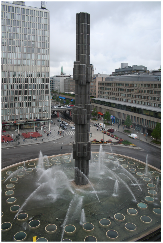
The Lamé curve became famous when it was proposed by the Danish mathematician and poet Piet Hein as an aesthetic and functional compromise between forms based on rectangular patterns and forms based on curvilinear patterns. In a design challenge for the city square Sergels Torg, in Stockholm, Piet Hein suggested a superellipse as an intermediate form between the traditional roundabout and a rectangular arrangement of roads, producing the result visible in this figure. Of all the superellipses, the most aesthetically perfect was, in Piet Hein’s opinion, the one parametrized by \(n=\frac{5}{2}\) and \(\frac{a}{b}=\frac{6}{5}\).

The superellipse-shaped fountain proposed by Piet Hein for the Sergels Torg square, in Stockholm. Photograph by Nozzman.

To draw the Lamé curve it is preferable to use the following parametric formulation:

\[\left\{ \begin{aligned} x\left(t\right) &= a\left(\cos^2 t\right)^{\frac{1}{n}} \cdot \operatorname{sgn} \cos t\\ y\left(t\right) &= b\left(\sin^2 t\right)^{\frac{1}{n}} \cdot \operatorname{sgn} \sin t \end{aligned}\right. \qquad -\pi \le t < \pi\]

The translation of this formula to Julia is straightforward:

superellipse(p, a, b, n, t) =

p+vxy(a*(cos(t)^2)^(1.0/n)*sign(cos(t)), b*(sin(t)^2)^(1.0/n)*sign(sin(t)))

In order to generate a sequence of points of the superellipse we can, as previously, use the map_division function:

superellipse_points(p, a, b, n, pts) =

map_division(t -> superellipse(p, a, b, n, t), -pi, pi, pts, _false)

Finally, to draw the superellipse, we can define:

superellipse_curve(p, a, b, n, pts) =

closed_spline(superellipse_points(p, a, b, n, pts))

The superellipses in this figure were generated using the previous function. For this, we defined the function test_superellipses that receives the values of \(a\) and \(b\) and a sequence of numbers, and tests all the combinations of exponent \(n=p/q\), with \(p\) and \(q\) taking successive values from that sequence. Each superellipse has an origin proportional to the combination of \(p\) and \(q\):

test_superellipses(a, b, ns) =

for num in ns

for den in ns

superellipse_curve(xy(num*2.5*a, den*2.5*b), a, b, num/den, 100)

end

end

This figure was directly generated from the evaluation of the following expression:

test_superellipses(2.0, 1.0, [1, 2, 3, 4, 5, 6, 7, 8])

10.3.7 Exercises 50

10.3.7.1 Question 182

Define the function superellipse_wall that creates a superellipse-shaped wall identical to the one of Sergels Torg fountain, as presented below:

Suggestion: define a function named curved_wall that builds walls along a given curve. The function should receive the thickness and height of the wall and an entity representing the curve (e.g., a circle, a spline, etc.). Also, consider using the sweep function defined in section Extrusion Along a Path.

10.3.7.2 Question 183

Define the function circular_walls that builds a succession of circular walls whose centers are located along a superellipse, as presented in the following image:

The function should receive the parameters of the superellipse, the parameters of a circular wall, and the number of walls to create.

10.3.7.3 Question 184

Define a function that, by invoking the functions superellipse_wall and circular_walls, creates a model as similar as possible to Sergels Torg’s fountain, as shown in the following figure:

10.3.7.4 Question 185

Modify the previous function to produce a variant that is perfectly circular:

10.3.7.5 Question 186

Modify the previous function to produce the following variant:

10.3.7.6 Question 187

Modify the previous functions to produce the following variant: