7.5 Extrusions

We saw in the previous sections that Khepri provides a set of predefined solids, such as spheres, cuboids, and pyramids. Through the composition of those solids it is possible to model far more complex shapes. Still, in any case, these shapes will always be decomposable into the original basic solids.

Unfortunately, many of the shapes that our imagination can conceive are not easy to build from just the compositions of predefined solids. For example, consider the Kunst- und Ausstellungshalle der Bundesrepublik Deutschland (in short, the Bundeskunsthalle), an art and exhibition center designed by the Viennese architect Gustav Peichl. This building’s plan has a square shape, but one of its corners is cut by a sinusoid, as illustrated in this figure.

A detail of the Bundeskunsthalle in Bonn, Germany. Photograph by Hanneke Kardol.

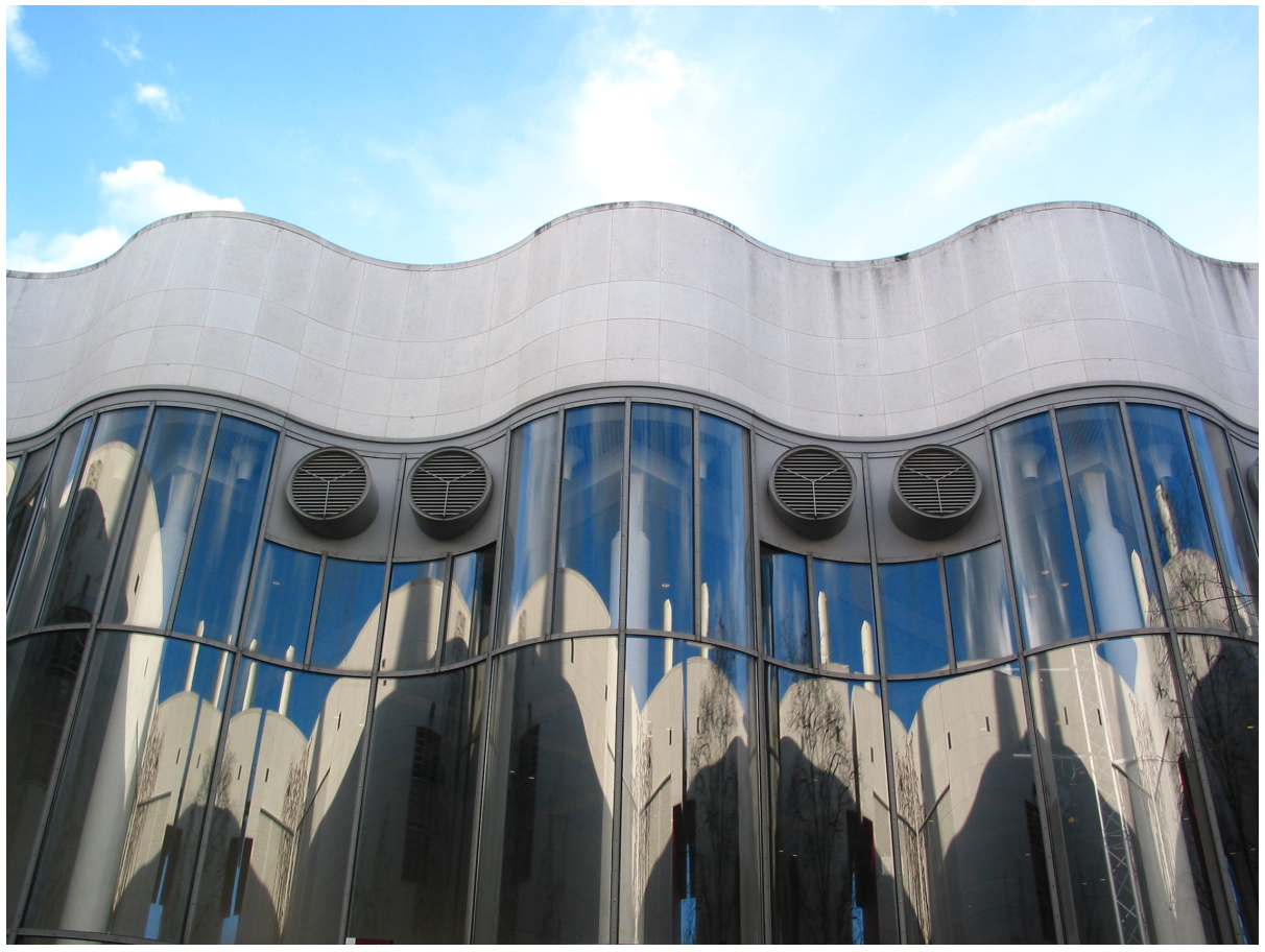
Obviously, to model the wavy wall of the Bundeskunsthalle, there is no predefined solid that we can use as a starting point for its construction.

Fortunately, Khepri provides a set of functionalities that allows us to easily solve some of these modeling problems. In this section, we will consider two of those functionalities, in particular, the simple extrusion and the extrusion along a path.

7.5.1 Simple Extrusion

Mechanically speaking, extrusion is a manufacturing process that consists in forcing a moldable material through a die with the desired section shape.

In Khepri, extrusion is an operation metaphorically identical to the one used in manufacturing. It is provided by the extrusion function, which receives as arguments the section shape to extrude and the direction of the extrusion, or the height if that direction is vertical. The resulting shape has the exact same section of the original shape.

The extrusion operates by virtually moving all the points of the region to extrude along the extrusion direction. As a result, when the region to extrude is a curve, the extrusion produces a surface, and when the region to extrude is a surface, the extrusion produces a solid. It is important to keep in mind that there are limitations to the process of extrusion, which prevent it from producing excessively complex shapes.

As an example, consider this figure where an arbitrary polygon lying in the \(XY\) plane is shown. This polygon can be created by the following expressions:

vertices = [xy(0, 2), xy(0, 5), xy(5, 3), xy(13, 3),

xy(13, 6), xy(3, 6), xy(6, 7), xy(15, 7),

xy(15, 2), xy(1, 2), xy(1, 0)]

polygon(vertices)

An arbitrary polygon.

To create a solid with a height of one from the extrusion of this polygon in the \(Z\) direction we can use the following expression:

extrusion(surface_polygon(vertices), vz(1))

The resulting shape is represented on the top of this figure. In the same figure, on the bottom, is represented an alternative extrusion that, instead of producing a solid, produces a surface. This extrusion can be obtained by replacing the previous expression with:

extrusion(polygon(vertices), vz(1))

A solid (on the left) and a surface (on the right) produced by the extrusion of, respectively, a polygonal surface and a polygon.

As another example, consider this figure, which illustrates two stylized flowers. The one on the top was produced using a set of cylinders with the base set at the same position and the top positioned along the surface of a sphere. The one on the bottom was produced by a set of extrusions from the same horizontal circular surface, using directions pointing along the surface of the sphere. As we can see, the extrusions of the circular surface in directions that are not perpendicular to that surface produce distorted cylinders.

A flower produced by a set of cylinders (above) and a flower produced by a set of extrusions (below).

Likewise, it is possible to extrude more complex planar shapes. For example, to create the sinusoidal wall of the Bundeskunsthalle, we can generate a surface on the \(XY\) plane from two parallel sinusoids and two line segments at their endpoints. Afterwards, we extrude the surface to the intended height, as represented in this figure.

Model of the Bundeskunsthalle’s sinusoidal wall.

This description can be translated to Julia:The sine_points function was defined in the section Polygonal Lines and Splines.

let pts_1 = sine_points(xy(0, 0), 0, 9*pi, 0.2),     pts_2 = sine_points(xy(0, 0.4), 0, 9*pi, 0.2)   extrusion(surface(spline(pts_1),                   spline(pts_2),                   spline([pts_1[1], pts_2[1]]),                   spline([pts_1[end], pts_2[end]])),             12) end

Although the result is a reasonable approximation to the Bundeskunsthalle’s wall, the used sinusoid is not parametrized enough to be adaptable to other situations of sinusoidal walls.

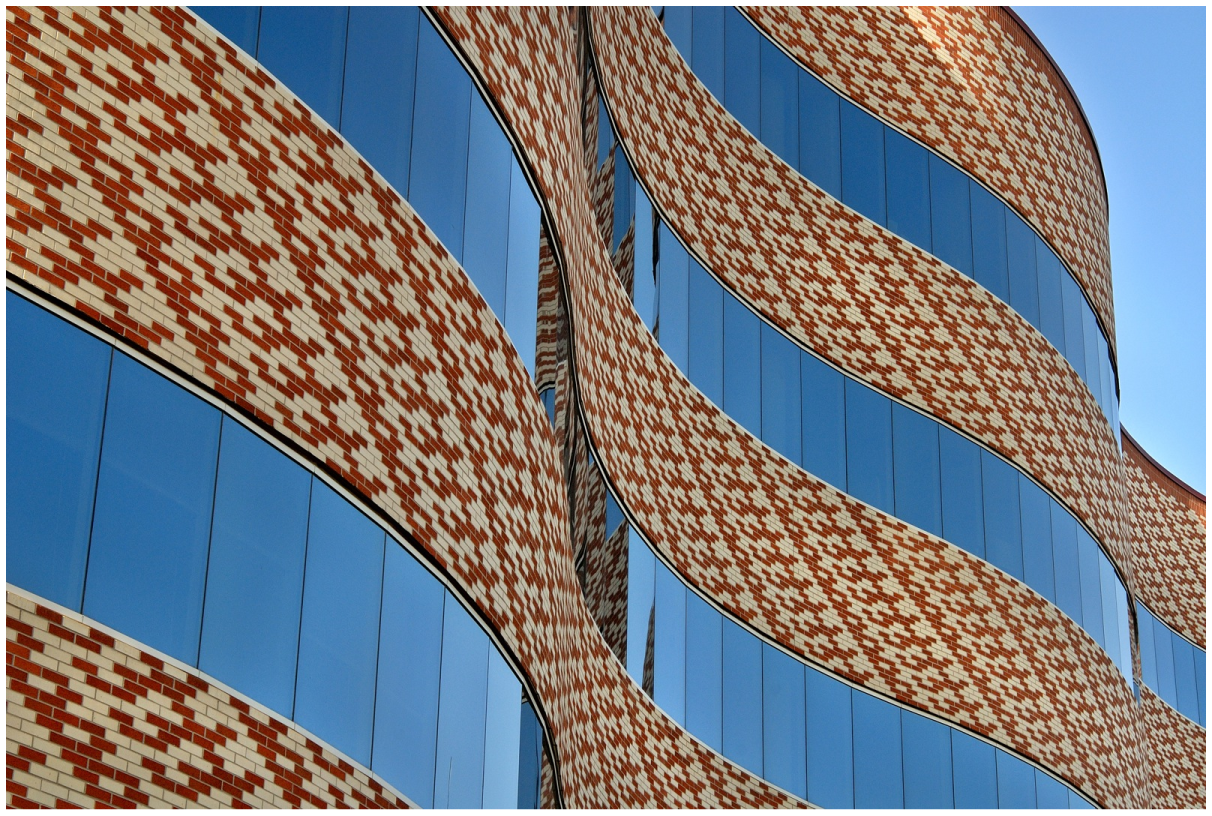
For example, in this figure we present a detail of the facade of a building in Tucson, Arizona. Although the building has a sinusoidal shape, the parameters are different from the ones used for the Bundeskunsthalle.

Sinusoidal facade of a building in Tucson, Arizona. Photograph by Janet Little.

In order to model both presented examples, we need to find a formula for the sinusoid curve that is sufficiently parametrized. Mathematically, the sinusoid equation is:

\[y(x) = a \sin(\omega x + \phi)\]

where \(a\) is the amplitude of the sinusoid, \(\omega\) is the angular frequency, i.e., the number of cycles by length, and \(\phi\) is the phase, i.e., the advance or delay of the curve towards the \(Y\) axis. This figure shows a sinusoid curve, illustrating the meaning of these parameters.

Sinusoid curve.

The translation of the previous definition to Julia is as follows:

sinusoid(a, omega, phi, x) = a*sin(omega*x+phi)

The next step for modeling sinusoid curves is the definition of a function that produces an array of coordinates corresponding to the points of the sinusoid curve in an interval \([x_0,x_1]\), and separated by an increment \(\Delta_x\). Since we might be interested in producing sinusoid curves with the origin at a specific point \(P\), it is convenient that the function also includes that point as a parameter:

sinusoid_points(p, a, omega, phi, x0, x1, dx) =   if x0 > x1     []   else     [p+vxy(x0, sinusoid(a, omega, phi, x0)),      sinusoid_points(p, a, omega, phi, x0+dx, x1, dx)...]   end

Note that the generated points are all set on a plane parallel to the \(XY\) plane, with the sinusoid evolving in a direction parallel to \(X\) axis. This figure shows three sinusoids with different amplitudes and periods, obtained through the following expressions:

spline(sinusoid_points(xy(0, 0), 0.2, 1, 0, 0, 6*pi, 0.4))

spline(sinusoid_points(xy(0, 4), 0.4, 1, 0, 0, 6*pi, 0.4))

spline(sinusoid_points(xy(0, 8), 0.6, 2, 0, 0, 6*pi, 0.2))

Three sinusoid curves.

To build a sinusoidal wall, we only need to create two parallel sinusoids with a distance between them equal to the thickness \(t\) of the wall. These curves will then be closed to form a region that will be extruded to a certain height \(h\):

sinusoidal_wall(p, a, omega, phi, x0, x1, dx, t, h) =   let pts_1 = sinusoid_points(p, a, omega, phi, x0, x1, dx),       pts_2 = sinusoid_points(p+vy(t), a, omega, phi, x0, x1, dx)     extrusion(surface(spline(pts_1),                   spline(pts_2),                   spline([pts_1[1], pts_2[1]]),                   spline([pts_1[end], pts_2[end]])),               h)   end

7.5.2 Exercises 36

7.5.2.1 Question 138

Consider the extrusion of a random closed curve as exemplified in the following figure:

Each curve is a spline produced with points generated by the random_circle_points function defined in the exercise of Question 104. Write an expression capable of generating a solid similar to the ones presented in the previous image.

7.5.2.2 Question 139

Write an expression capable of creating a sequence of floors with a random shape, similar to the ones presented in the following example:

7.5.2.3 Question 140

Redo the previous exercise in order to make the floor sequence resemble a semi-sphere, as presented in the following image:

7.5.2.4 Question 141

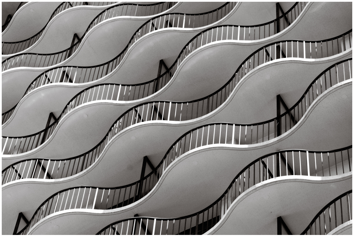
This figure shows a detail of the Hotel Marriott’s facade in Anaheim. It is observable that the balconies have a sinusoidal shape with equal amplitude and frequency, but alternating phases.

Detail of Hotel Marriott in Anaheim. Photograph by Abbie Brown.

Create a function called slab that receives all the parameters needed to generate a sinusoid and that creates a rectangular slab with one side having a sinusoidal shape, as presented in the following image:

The function should have the following parameters, which are illustrated in the figure below:

slab(p, a, omega, phi, ls, dx, ws, hs)

The parameter dx represents the increment \(\Delta_x\) to consider for the creation of the sinusoid’s points. The parameters ls, ws, and hs correspond, respectively, to the length, width, and height of the slab.

As an example, the previously represented slab was generated by the expression:

slab(xy(0, 0), 1.0, 1.0, 0, 2*pi, 0.5, 2, 0.2)

7.5.2.5 Question 142

Create a function called handrail that creates a sinusoidal handrail with a rectangular section, as presented in the following image:

The function should have the following parameters:

handrail(p, a, omega, phi, ls, dx, l_handrail, h_handrail)

The first parameters are needed to completely specify the sinusoid curve, whereas l_handrail and h_handrail correspond to the length and height of the rectangular section of the handrail.

For example, the previous image could have been generated by the expression:

handrail(xy(0, 0), 1.0, 1.0, 0, 2*pi, 0.5, 0.06, 0.02)

7.5.2.6 Question 143

Create a function called balusters that creates the supporting balusters for a sinusoidal handrail, as presented in the following image:

Notice that the balusters have a circular section and, therefore, have a cylindrical shape. Also note that the balusters have a certain distance dx between them.

The function should have the following parameters:

balusters(p, a, omega, phi, ls, dx, h_balusters, r_balusters)

The first parameters are necessary to completely specify the sinusoid curve, whereas the last two correspond to the height and radius of each cylinder.

For example, the previous image was generated by the expression:

balusters(xy(0, 0), 1.0, 1.0, 0, 2*pi, 0.5, 1, 0.02)

7.5.2.7 Question 144

Create a function called balustrade that, given the necessary parameters to create the handrail and the balusters, creates a balustrade, as the one shown in the following image:

To simplify, consider that the balusters have a diameter equal to the length of the handrail.

The function should have the following parameters:

balustrade(p, a, omega, phi, ls, dx,

h_balusters, l_handrail, h_handrail, d_balusters)

Once more, the first parameters completely specify the sinusoid curve. The parameters h_balusters, l_handrail, h_handrail and d_balusters specify, respectively, the height of the balusters, the length and height of the square section of the handrail and the horizontal displacement of the balusters.

For example, the previous image was generated by the expression:

balustrade(xy(0, 0), 1.0, 1.0, 0, 2*pi, 0.5, 1, 0.06, 0.02, 0.4)

7.5.2.8 Question 145

Create a function called floor that, given the parameters that characterize a slab and a balustrade, creates a floor, as illustrated in the following image:

To simplify, consider that the balustrade is positioned at the extremity of the slab. The function floor should have the following parameters:

floor(p, a, omega, phi, ls, dx, ws, hs,

h_balusters, l_handrail, h_handrail, d_balusters)

For example, the previous image resulted from the expression:

floor(xy(0, 0), 1.0, 1.0, 0, 2*pi, 0.5, 2, 0.2, 1, 0.06, 0.02, 0.4)

7.5.2.9 Question 146

Create a function called building that receives all the necessary parameters to create a floor, including the height of each floor h_floor and the number of floors n_floors, and creates a building similar to the one presented in the following image:

The function building should have the following parameters:

building(p, a, omega, phi, ls, dx, ws, hs,

h_balusters, l_handrail, h_handrail, d_balusters, h_floor, n_floors)

For example, the previous image could have been generated by the following expression:

building(xy(0, 0), 1.0, 1.0, 0, 20*pi, 0.5, 20, 0.2, 1, 0.06, 0.02, 0.4, 4, 8)

7.5.2.10 Question 147

Modify the building function to receive an additional parameter that represents a phase increment to be considered at each floor. That parameter makes it possible to generate buildings with more interesting facades, where the floors’ sinusoidal shapes are displaced from each other. For example, compare the following building with the previous one:

7.5.2.11 Question 148

The following images illustrate some variations of the phase increment. Identify the increment used in each example.

7.5.3 Extrusion Along a Path

So far, extrusions create solids (or surfaces) through the movement of a section along a direction. With the sweep function, it is possible to generalize this process so that the movement is made along an arbitrary curve. As with simple extrusion, it is important to keep in mind that there are limitations to the extrusion process that prevent it from creating excessively complex forms or using excessively complex paths.

As an example, consider the creation of a cylindrical tube with a sinusoidal shape, as the one illustrated in this figure. It is noticeable that the section to extrude is a circle and that the extrusion cannot be performed over a fixed direction, otherwise the result will not have the intended sinusoidal shape. So, instead of extruding a circle along a line, we can simply move that circle along a sinusoid. The example provided in this figure was produced by the following expression:

A cylindrical tube with a sinusoidal shape.

let section = surface_circle(xy(0, 0), 0.4),     curve = spline(sinusoid_points(xy(0, 0), 1, 1, 0, 0, 7*pi, 0.2))   sweep(curve, section) end

Both the extrusion along a path (sweep) and the simple extrusion (extrusion) allow the creation of countless types of solids. However, it is important to know which operation is best suited for each case. As an example, consider once more the creation of a sinusoidal wall. In section Simple Extrusion we did it by vertically extruding a region limited by two sinusoids. Unfortunately, when the sinusoids have accentuated curvatures, the resulting walls will have a thickness that is clearly non-uniform, as exemplified by the thicker profile presented in this figure.

Top view of two overlapping sinusoidal walls. The thicker profile was generated from the extrusion of a region limited by two sinusoids. The thinner profile was generated by the extrusion of a rectangular region along a sinusoid.

To give the wall a uniform thickness (as exemplified by the thinner profile of this figure), it is preferable to model the wall as a rectangle (dimensioned by the height and thickness), which moves along the curve that constitutes the central axis the wall. This is implemented in the following function:

sinusoidal_wall(p, a, omega, phi, x0, x1, dx, height, thickness) =   sweep(spline(sinusoid_points(p+vxyz(0, thickness/2.0, height/2.0),                        a,                        omega,                        phi,                        x0,                        x1,                        dx)),         surface_rectangle(xy(-thickness/2.0, -height/2.0), thickness, height))

The previous function easily allows us to create the intended walls. The following expressions were used to generate this figure.

sinusoidal_wall(xy(0, 0), 0.2, 1, 0, 0, 6*pi, 0.4, 3, 0.2)

sinusoidal_wall(xy(0, 4), 0.4, 1, 0, 0, 6*pi, 0.4, 2, 0.4)

sinusoidal_wall(xy(0, 8), 0.6, 2, 0, 0, 6*pi, 0.2, 5, 0.1)

Three walls with different heights and thicknesses and shaped by sinusoid curves.

7.5.4 Exercises 37

7.5.4.1 Question 149

Redo the exercise of Question 142 by using an extrusion along a path.

7.5.4.2 Question 150

Define a function wall_points that, given the thickness and height of a wall and a curve described by an array of points, builds a wall by sweeping a rectangular section, with the given thickness and height, through a spline that goes through the given coordinates. If needed, you can use the spline function which, from an array of points, creates a spline that goes through those points.

7.5.5 Extrusion with Transformation

The operation of extrusion along a path provided by Khepri also allows us to apply transformations to the section as it is being extruded. The available transformations are the rotation (which is particularly useful to model shapes with torsions) and the scale. Both rotation angle and scale factor are optional parameters of the sweep function.

As an example, consider the modeling of the columns presented in the building represented in this figure.

Twisted columns on the facade of a building in Atlanta. Photograph by Pauly.

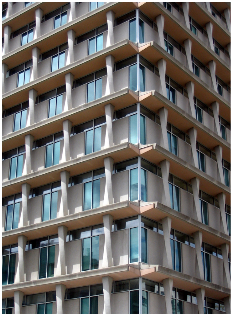
Since these columns correspond to cuboids to which a torsion of \(90^o\) was applied, we can simulate this shape by extruding a square section while rotating it \(90^o\) during the extrusion process:

sweep(line(u0(), z(30)),       surface_polygon(xy(-1, -1), xy(1, -1), xy(1, 1), xy(-1, 1)),       pi/2)

To better understand the torsion effect, this figure illustrates the torsion process of columns with a square section, in successive angle increments of \(\frac{\pi}{4}\), from a torsion of \(2\pi\) clockwise to a torsion of \(2\pi\) in the opposite direction.

Square section columns twisted in increments of \(\frac{\pi}{4}\) radians.