10.6 Parametric Surfaces

Throughout history, architecture has explored a huge variety of shapes. As we saw, some of these shapes correspond to solids well known since antiquity, such as cubes, spheres and cones. More recently, architects have turned their attention to much less classical shapes, which require a different kind of description. The famous Spanish and Mexican architect Félix Candela is a good example.

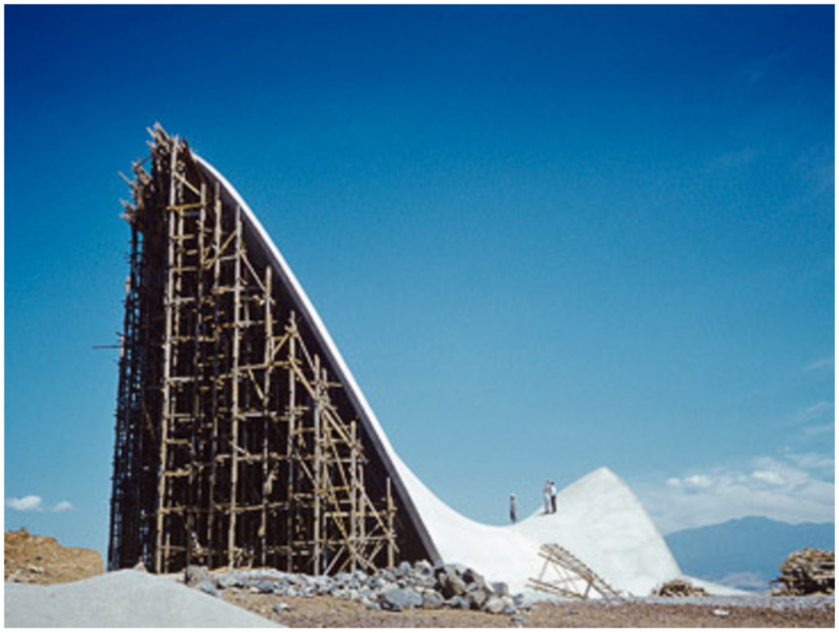
Candela thoroughly explored the properties of the hyperbolic paraboloid, allowing him to create works that are now references in the world of architecture. This figure illustrates the construction of one of the works of Félix Candela, where the fundamental element is precisely a thin concrete shell in the shape of a hyperbolic paraboloid.

The Chapel Lomas de Cuernavaca under construction. Photograph by Dorothy Candela.

Candela manually performed all necessary calculations to determine the shapes he intended to create. We will now see how we can get the same results in a much more efficient way.

For this, we are going to generalize the parametric description of curves to the parametric description of surfaces. Even though a three-dimensional curve is described by a triplet of functions of a single parameter \(t\), for example, \((x(t), y(t), z(t))\), a surface will have to be described by a triplet of functions of two parameters that vary independently, Mathematically speaking, a parametric surface is simply the image of an injective function that maps \(\mathbb R^2\) into \(\mathbb R^3\). for example, \((x(u,v), y(u,v), z(u,v))\). Naturally, the choice between rectangular, cylindrical, and spherical coordinates, among others, is just a matter of convenience: in any case, three functions are required.

As it happens with curves, although we can describe a surface in an implicit form, the parametric representation is more adequate for the generation of the positions through which the surface passes. For example, a sphere centered at the point \((x_0, y_0, z_0)\) and with radius \(r\) can be described implicitly by the equation

\[(x-x_0)^2+(y-y_0)^2+(z-z_0)^2-r^2=0\]

However, this form does not allow the direct generation of coordinates. Thus, it is preferable to adopt a parametric description, given by the functions

\[\left\{ \begin{aligned} x(\phi,\psi) &= x_0 + r \sin\phi\cos\psi\\ y(\phi,\psi) &= y_0 + r \sin\phi\sin\psi\\ z(\phi,\psi) & =z_0 + r \cos\phi \end{aligned}\right.\]

10.6.1 The Möbius Strip

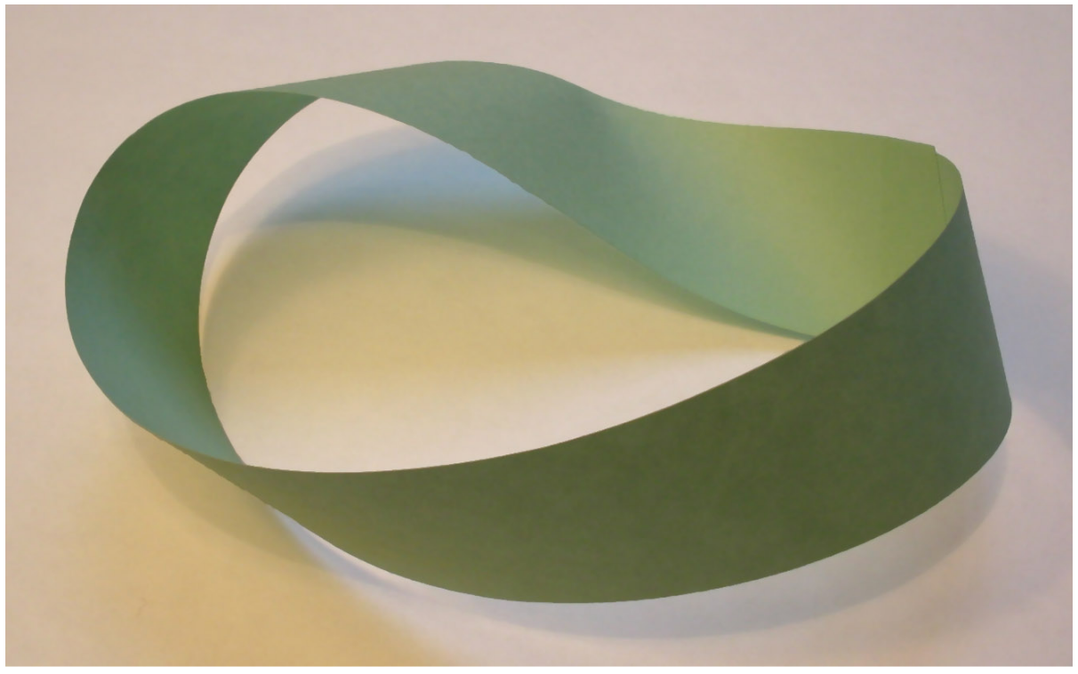
To illustrate the concept of parametric surface, we are going to consider a famous surface: the Möbius strip. The Möbius strip is not a true surface, but a surface with boundary.

The Möbius strip (also known as Möbius band) was independently described by two German mathematicians in 1858, first by Johann Benedict Listing and, two months later, by August Ferdinand Möbius. Although Listing was the only one who published his discovery, it was eventually baptized with the name of Möbius.

This figure shows a picture of a Möbius strip made from a half-twisted paper band. With it, we can see one of the extraordinary features of this surface: it is possible to go all the way around the surface without ever leaving the same side because, in truth, the Möbius strip only has one side. The properties of the Möbius strip have been exploited, for example, in conveyor belts that, when adopting the topology of a Möbius strip, wear out the entire surface instead of only one side, thereby making them last twice as long. Likewise, the surface is limited only by one edge. In fact, the Möbius strip is the simplest surface of only one side and one edge.

The Möbius strip.

The Möbius strip has been used in various contexts, from the famous artworks of Maurits Cornelis Escher that employ a Möbius strip, such as the "Möbius Strip II", to the recycling symbol, which consists of three arrows arranged along a Möbius strip, as can be seen in this figure.

The recycling symbol: three arrows arranged along a Möbius strip.

The parametric equations of this surface, in cylindrical coordinates, are as follows:

\[\left\{ \begin{aligned} \rho(u,v)& =1 + v \cos\frac{u}{2}\\ \phi(u,v)& =u\\ z(u,v)& =v \sin\frac{u}{2} \end{aligned}\right.\]

Given the periodicity of the trigonometric functions, we have that \(\frac{u}{2} \in [0,2\pi]\) or \(u \in [0,4\pi]\). In that period, for a given \(v\), the \(z\) coordinate will assume symmetrical values in relation to the \(xy\) plane, in the limit, between \(-v\) and \(v\). This means that the Möbius strip develops up and down the \(xy\) plane.

To draw this surface we can use, as an initial approach, a generalization of the process we used to draw parametric curves. In that case, we applied the argument function \(f(t)\) along a succession of \(n\) values ​​from \(t_0\) to \(t_1\). In the case of parametric surfaces, we will apply the function \(f(u,v)\) along a succession of \(m\) values ​​from \(u_0\) to \(u_1\), and, for each one, along a succession of \(n\) values from \(v_0\) to \(v_1\). Thus, the \(f(u,v)\) function will be applied to \(m\times n\) values. This behavior can be obtained by two chained mappings:

map(u -> map(v -> f(u, v), division(v0, v1, n)),     division(u0, u1, m))

For example, in the case of Möbius strip, we can define:

mobius_strip(u0, u1, m, v0, v1, n) =

map(u -> map(v -> cyl(1+v*cos(u/2), u, v*sin(u/2)), division(v0, v1, m)),

division(u0, u1, n))

In reality, this combination of mappings with interval divisions is so frequent that Khepri already provides it through the map_division function itself, allowing us to write

mobius_strip(u0, u1, m, v0, v1, n) =

map_division((u, v) -> cyl(1+v*cos(u/2), u, v*sin(u/2)), u0, u1, m, v0, v1, n)

We have seen that in the case of a function with a single parameter \(f(t)\), we had

map(unsyntax(lispemph(f)),     division(lispemphi(t, "0"), lispemphi(t, "1"), unsyntax(lispemph(n))))

This equivalence is now extended to the case of functions that have two parameters \(f(u,v)\), that is,

map_division(unsyntax(lispemph(f)),              lispemphi(u, "0"),              lispemphi(u, "1"),              unsyntax(lispemph(n)),              lispemphi(v, "0"),              lispemphi(v, "1"),              unsyntax(lispemph(m)))

is equivalent to

map(u -> map(v -> unsyntax(lispemph(f))(u, v), division(lispemphi(v, "0"), lispemphi(v, "1"), unsyntax(lispemph(m)))),     division(lispemphi(u, "0"), lispemphi(u, "1"), unsyntax(lispemph(n))))

Naturally, if the interior mapping produces an array with the results of the application of the function \(f\), the exterior mapping will produce an array of arrays of results of the application of the function \(f\). Assuming that each application of the function \(f\) yields a position in three-dimensional coordinates, the previous expression produces an array of arrays of positions in the following format:

lispemphi(P, "0,0")(lispemphi(P, "0,1"), ___, lispemphi(P, "0,m"))(lispemphi(P, "1,0")(lispemphi(P, "1,1"),                                                                                        ___,                                                                                        lispemphi(P,                                                                                                  "1,m")),                                                                    ___,                                                                    lispemphi(P, "n,0")(lispemphi(P, "n,1"),                                                                                        ___,                                                                                        lispemphi(P,                                                                                                  "n,m")))

To visualize this array of arrays of positions, we can simply apply the spline function to each of the arrays of positions:

splines(ptss) = map(spline,

ptss)

Thus, we can easily represent a first preview of the Möbius strip:

splines(mobius_strip(0, 4*pi, 80, 0, 0.3, 10))

The result of the evaluation of the above expression is represented in this figure.

The Möbius strip represented by transversal splines.

An interesting aspect of three-dimensional parametric surfaces is that the set of points that define them can be arranged in a matrix. In fact, if the parametric surface is obtained by applying the function \(f(u,v)\) over a succession of \(n\) values from \(u_0\) to \(u_1\), and, for each one, over a succession of \(m\) values ​​from \(v_0\) to \(v_1\), we can place the results of those applications in a matrix of \(m\) rows and \(n\) columns, as follows:

\[\begin{bmatrix} f(u_0,v_0) & \dots & f(u_0,v_1)\\ \dots & \dots & \dots\\ f(u_1,v_0) & \dots & f(u_1,v_1) \end{bmatrix}\]

What the map_division function returns is a representation of this matrix, implemented as an array of matrix rows, being each row implemented as an array of elements.

It is now easy to see that the function splines draws \(m\) splines, each defined by \(n\) points of each \(m\) matrix rows. Another alternative is to draw \(n\) splines defined by \(m\) points of each \(n\) matrix columns. For this, the simplest way is to transpose the matrix, i.e., to switch the rows with the columns, in the form:

\[\begin{bmatrix} f(u_0,v_0) & \dots & f(u_1,v_0)\\ \dots & \dots & \dots\\ f(u_0,v_1) & \dots & f(u_1,v_1) \end{bmatrix}\]

To implement this operation, we can define a function that, given a matrix represented as an array of arrays, returns the transposed matrix in the same representation:

transposed_matrix(matrix) =

matrix[1] == [] ?

[] :

[map(l -> l[1], matrix), transposed_matrix(map(l -> l[2:end], matrix))...]

Using this function, it is now possible to draw orthogonal curves to the ones represented in this figure simply by drawing splines obtained from the transposed matrix, i.e.:

splines(transposed_matrix(mobius_strip(0, 4*pi, 80, 0, 0.3, 10)))

The result of evaluating this expression is shown in this figure.

The Möbius strip represented by longitudinal splines.

Finally, to obtain a mesh with the combination of both curves, we can define an auxiliary function mesh_splines:

mesh_splines(ptss) =

begin

splines(ptss)

splines(transposed_matrix(ptss))

end

We can now use this function as follows:

mesh_splines(mobius_strip(0, 4*pi, 80, 0, 0.3, 10))

The result of evaluating this expression is shown in this figure.

The Möbius strip represented by a mesh of splines.

This type of representation, based on the use of lines to give the illusion of an object, is called wireframe. Formally, a wireframe is a set of lines that represent a surface. Wireframe models have the advantage, over other forms of visualization, of allowing a much faster calculation.