4.5 Recursion in Nature

Recursion is present in countless natural phenomena. A recursive process allows the generation of self-similar patterns (in which the whole has a shape similar to a part of itself). Those patterns are visible in many apparent chaotic structures. Mountains, for example, exhibit irregularities that when observed at an appropriate scale are identical to... mountains. A river has tributaries and each tributary is identical to... a river. A blood vessel has branches and each branch is identical to... a blood vessel. All these natural entities are examples of recursive structures.

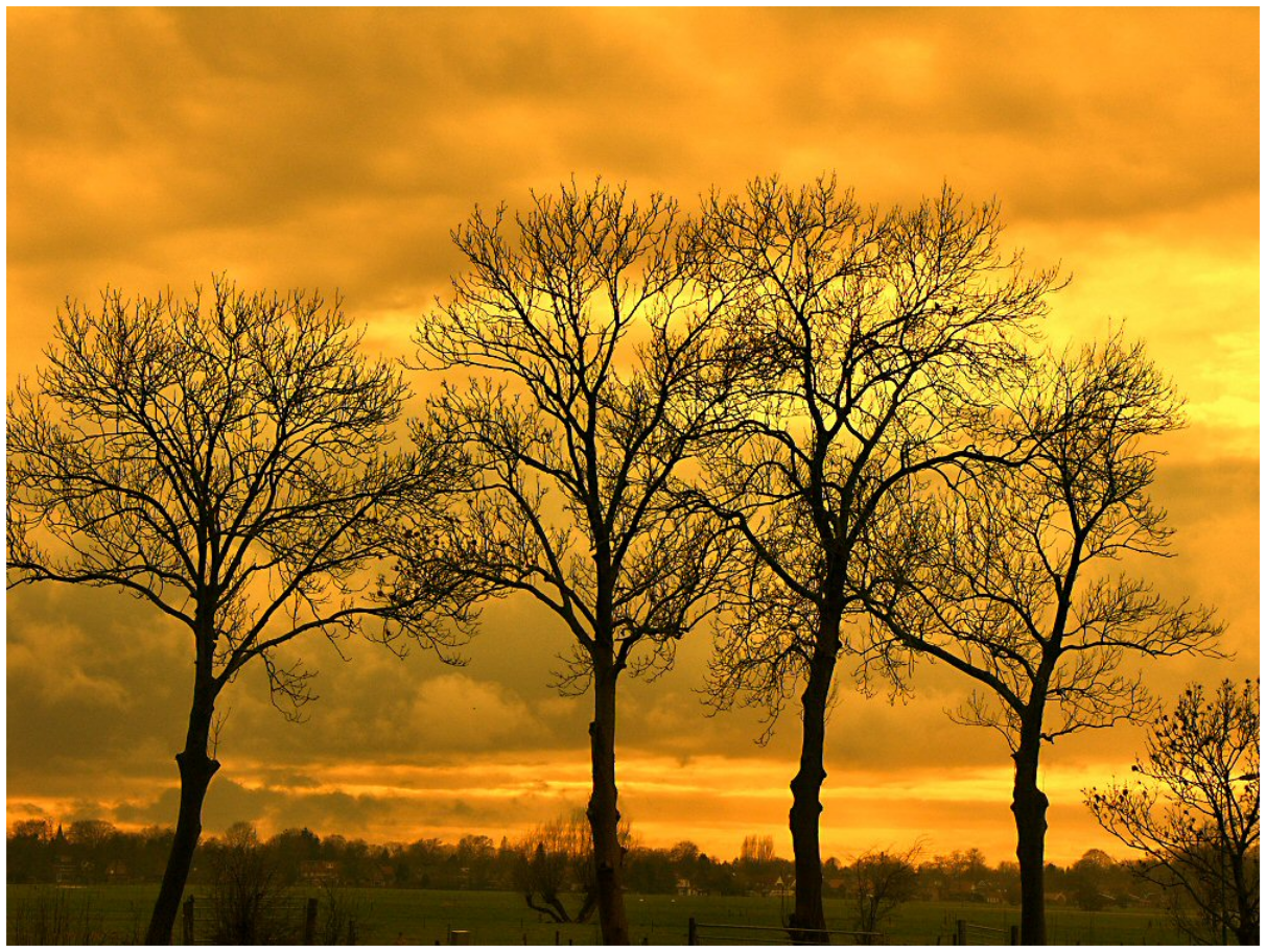
A tree is another good example of a recursive structure, since, as it can be seen in this figure, tree branches are similar to small trees growing from the trunk. Likewise, from each tree branch there are other small trees growing from them, a process that repeats itself until its dimension becomes sufficiently small and other structures appear, such as leaves, flowers, fruits, etc.

The recursive structure of trees. Photograph by Michael Bezzina.

If, in fact, a tree has a recursive structure, it should be possible to create trees with recursive functions. To test this theory, let us start by considering a very simplistic version of a tree, where we have a trunk that, at one certain point, is divided into two sub-trunks, or branches. Each of these branches grows with an angle from the main trunk, and reaches a certain length that is a fraction of the main trunk’s length, as shown in this figure. The stopping condition is reached when the length of the branch becomes so small that, instead of continuing dividing itself, a different structure appears. To simplify, let us consider that, at the extremity of the smaller branches, a leaf appears, which we will represent with a small circle.

Drawing parameters of a tree.

Let us consider a tree function that receives, as arguments, the position \(P\) of the tree base, the length \(l\) of the trunk and the angle \(\alpha\) of the trunk. For the recursive case, we will have as parameters the opening angle \(\Delta_\alpha\) that the new branch should make with the previous one, and the reduction factor \(f\) for the trunk’s length.

The first step is to compute the top of the trunk, which can be easily done with polar coordinates, and we draw the trunk from the base to the top. Next, we test if the drawn trunk is sufficiently small. If it is, we finish with the drawing of a circle centered at top. Otherwise, we make one recursive call to draw a sub-tree on the right and another to draw a sub-tree on the left. The definition of the function is then:

tree(p, l, a, da, f) =   let top = p+vpol(l, a)     branch(p, top)     if l < 0.2       leaf(top)     else       tree(top, l*f, a+da, da, f)       tree(top, l*f, a-da, da, f)     end   end

branch(p0, p1) = line(p0, p1)

leaf(p) = circle(p, 0.02)

A first example of a tree, created by the following code, is presented in this figure.

tree(xy(0, 0), 2, pi/2, pi/8, 0.7)

Drawing of a tree, whose trunk measures \(20\) units, with an initial angle of \(\frac{\pi}{2}\), an opening angle of \(\frac{\pi}{8}\) and a reduction factor of \(0.7\).

Other examples are presented in this figure, in which the opening angle and the reduction factor vary. The sequence of expressions that generated those examples is the following:

tree(xy(0, 0), 2, pi/2, pi/8, 0.6)

tree(xy(10, 0), 2, pi/2, pi/8, 0.8)

tree(xy(20, 0), 2, pi/2, pi/6, 0.7)

Various trees with different opening angles and reduction factors.

Unfortunately, the presented trees are "excessively" symmetrical: in nature it is literally impossible to find perfect symmetries. For this reason, the model should become a little bit more sophisticated, with the introduction of different growth parameters for the branches on the left and on the right. For that, instead of having a single opening angle and only one length reduction factor, we will apply two, as presented in this figure.

Drawing parameters of a tree with asymmetrical growth.

The redefinition of the tree function to receive the additional parameters is straightforward:

tree(p, l, a, da0, f0, da1, f1) =   let top = p+vpol(l, a)     branch(p, top)     if l < 0.2       leaf(top)     else       tree(top, l*f0, a+da0, da0, f0, da1, f1)       tree(top, l*f1, a-da1, da0, f0, da1, f1)     end   end

This figure presents new examples of trees with different opening angles and reduction factors on the left and right branches, which were generated by the following expressions:

tree(xy(0, 0), 2, pi/2, pi/8, 0.6, pi/8, 0.7)

tree(xy(8, 0), 2, pi/2, pi/4, 0.7, pi/16, 0.7)

tree(xy(15, 0), 2, pi/2, pi/6, 0.6, pi/16, 0.8)

Various trees generated with different opening angles and reduction factors for both left and right branches.

The trees generated by the tree function are only a poor model of reality. Although there are obvious signs that various natural phenomena can be modeled by recursive processes, nature is not as deterministic as our functions. So, in order to make our tree function closer to reality, it is crucial that some randomness is incorporated. This will be the subject of the next section.