4.4 Ionic Order
The Ionic order is one of the three classical orders of Greek architecture. The volute, an architectural element that characterizes the Ionic order, is a spiral-shaped ornament placed at the top of an Ionic capital. This figure shows an example of an Ionic capital containing two volutes. Although we still have numerous samples of volutes from antiquity, their drawing process was never clear.
Volutes of an Ionic capital. Photograph by See Wah Cheng.
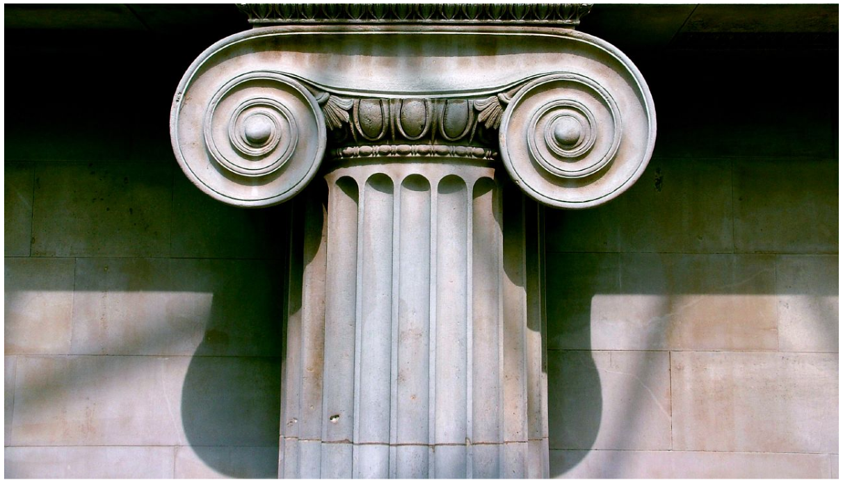
Vitruvius, in his architectural treatise, describes the Ionic volute: a spiral-shaped curve that starts at the base of the abacus, unfolds into a series of turns and joins with a circular element called the eye. Vitruvius describes the spiral drawing process through a composition of arcs, each covering a quarter of a circumference, starting at the outermost point and decreasing the arc radius one at a time, until joining with the eye. In his description, there are still some details to be explained, in particular, the position of the centers of the arcs. Vitruvius mentions that a calculation and a figure will be added at the end of the book, but, unfortunately, those were never found. The doubts regarding the drawing process of this element become even more evident when analysis performed on the many volutes that survived the antiquity revealed differences to the proportions described by Vitruvius.
During the Renaissance period, these doubts made researchers rethink Vitruvius’ method by suggesting personal interpretations or completely new methods for designing volutes. The more relevant methods are the ones proposed in the 16th century by Sebastiano Serlio (based on the composition of semi-circumferences), by Giuseppe Salviati (based on the composition of quarters of a circumference), and by Guillaume Philandrier (based on the composition of eighths of a circumference).
All those methods differ in many details but, generically, they are all based on the use of arcs of circumference with constant angle amplitude but with a decreasing radius. Obviously, to ensure continuity between the arcs, their centers must change as they are being drawn. This figure presents the process of drawing spirals using quarters of a circumference.
Drawing of a spiral using quarters of a circumference.

As shown in the figure above, in order to draw the spiral we must draw successive circumference arcs. The first arc is centered at the point \(P\) and has a radius \(r\). This first arc goes from the angle \(\pi/2\) to \(\pi\). The second arc is centered at the point \(P_1\) and has a radius of \(r\cdot f\), with \(f\) being the reduction factor of the spiral. This second arc goes from the angle \(\pi\) to \(\frac{3}{2}\pi\). An important detail is the relationship between the coordinates of \(P\) and \(P_1\): for the second arc starting point to be coincident with the first arc endpoint, its center must be the sum of \(P\) with the vector \(\vec{v}_0\), whose length is \(r\cdot(1-f)\), and whose direction is equal to the final angle of the first arc.
This process should be repeated for the remaining arcs to calculate the coordinates \(P_2\), \(P_3\), etc., as well as the radii \(r\cdot f \cdot f\), \(r\cdot f \cdot f \cdot f\), etc., which are needed to draw the remaining arcs.
Described this way, the drawing process seems complicated. However, it is possible to rewrite it so that it becomes much simpler, by thinking about the spiral as an arc followed by a smaller spiral. Therefore, a spiral centered at the point \(P\), with a radius \(r\), and an initial angle \(\alpha\), can be defined by an arc of radius \(r\), centered at \(P\), with an initial angle of \(\alpha\) and a final angle of \(\alpha + \frac{\pi}{2}\), followed by a spiral centered at \(P+\vec{v}\), with a radius of \(r\cdot f\) and an initial angle of \(\alpha + \frac{\pi}{2}\). The vector \(\vec{v}\) will have a length of \(r\cdot(1-f)\) and an angle of \(\alpha + \frac{\pi}{2}\).
Obviously, being this a recursive process, it is necessary to define the stopping condition, for which we have (at least) two possibilities:
End when the number of arcs is zero;
End when the radius \(r\) is smaller than a certain limit;
End when the angle \(\alpha\) is bigger than a certain limit.
For now, we will consider the first possibility. According to the described process, let’s define the function that draws the spiral with the following parameters: the p starting point, the r initial radius, the a initial angle, the n number of quarters of a circumference, and the f reduction factor:
spiral(p, r, a, n, f) =
if n == 0
nothing
else
circumference_quarter(p, r, a)
spiral(p+vpol(r*(1-f), a+pi/2), r*f, a+pi/2, n-1, f)
end
Note that the spiral function is recursive, as it is defined in terms of itself. Obviously, the recursive case is simpler than the original case, since the number of quarters of a circumference is smaller, progressively approaching the stopping condition.
To draw each arc we will use Khepri’s arc function which receives the arc’s center, radius, initial angle, and angle amplitude. To visualize the drawing process, we will also draw two lines starting at the arc’s center and ending in its endpoints. Later, once we have finished developing these functions, we will remove them.
circumference_quarter(p, r, a) =
begin
arc(p, r, a, pi/2)
line(p, p+vpol(r, a))
line(p, p+vpol(r, a+pi/2))
end
Now we can test an example:
spiral(xy(0, 0), 3, pi/2, 12, 0.8)
The spiral drawn by the expression above is shown in this figure.
A spiral composed by quarters of a circumference.

The spiral function allows us to define any number of spirals, but with one restriction: each circular arc corresponds to an angle increment of \(\frac{\pi}{2}\). Obviously, this function would be more useful if this increment was also a parameter, as shown in this figure.
Spiral with the angle increment as a parameter.

As can be deduced from observing the figure above, the required modifications are relatively simple. We only need to add the parameter da, representing the angle increment \(\Delta_\alpha\) of each arc, and replace the occurrences of \(\frac{\pi}{2}\) with it. Naturally, instead of always drawing a quarter of a circumference, we will now draw an arc of angle amplitude \(\Delta_\alpha\). Since the use of this parameter also affects the meaning of the parameter \(n\), which now represents the number of arcs with that amplitude, it is advisable to explore a different stopping condition based on the intended final angle fa. However, we need to consider one final detail: the last arc may not be a complete arc if the difference between the final and initial angle is smaller than the angle amplitude \(\Delta_\alpha\). In this case, the arc will only have this difference as angle amplitude. The new definition is then:
spiral(p, r, a, da, fa, f) =
if fa-a < da
spiral_arc(p, r, a, fa-a)
else
spiral_arc(p, r, a, da)
spiral(p+vpol(r*(1-f), a+da), r*f, a+da, da, fa, f)
end
The function that draws the arc is a generalization of the one that draws one quarter of a circumference:
spiral_arc(p, r, a, da) =
begin
arc(p, r, a, da)
line(p, p+vpol(r, a))
line(p, p+vpol(r, a+da))
end
Right now, to draw the spiral previously represented in this figure, we have to evaluate the following expression:
spiral(xy(0, 0), 3, pi/2, pi/2, pi*6, 0.8)
Noticeably, we can now easily draw other spirals. The spirals produced by the following expressions, comprising different reduction factors, are shown in this figure:
spiral(xy(0, 0), 2, pi/2, pi/2, pi*6, 0.9)
spiral(xy(4, 0), 2, pi/2, pi/2, pi*6, 0.7)
spiral(xy(8, 0), 2, pi/2, pi/2, pi*6, 0.5)
Various spirals with different reduction factors: \(0.9\), \(0.7\) and \(0.5\), respectively.

Another possibility is to change the angle increment. The following expressions test approximations to Sebastiano Serlio’s approach (semi-circumferences), Giuseppe Salviati’s approach (circumference-quarters) and Guillaume Philandrier’s approach (circumference-eights), respectively: Note that these are mere approximations. The original methods were much more complex.
spiral(xy(0, 0), 2, pi/2, pi, pi*6, 0.8)
spiral(xy(4, 0), 2, pi/2, pi/2, pi*6, 0.8)
spiral(xy(8, 0), 2, pi/2, pi/4, pi*6, 0.8)
The results of evaluating the previous expressions are shown in this figure.
Various spirals with a reduction factor of \(0.8\) and different angle increments: \(\pi\), \(\frac{\pi}{2}\), and \(\frac{\pi}{4}\), respectively.

Finally, in order to compare the drawing process of the different spirals, we should adjust the reduction factor to the angle increment, so that the reduction is applied to one whole turn and not just to the chosen angle increment. Thus, we have the following expressions:
spiral(xy(0, 0), 2, pi/2, pi, pi*6, 0.8)
spiral(xy(4, 0), 2, pi/2, pi/2, pi*6, 0.8^(1/2))
spiral(xy(8, 0), 2, pi/2, pi/4, pi*6, 0.8^(1/4))
The results of evaluating the previous expressions are shown in this figure.
Various spirals with a reduction factor of \(0.8\) per turn and with different angle increments: \(\pi\), \(\frac{\pi}{2}\) and \(\frac{\pi}{4}\), respectively.

4.4.1 Exercises 26
4.4.1.1 Question 74
The golden spiral is a spiral whose growth factor is the golden ratio \(\varphi\), being \(\varphi=\frac{1 + \sqrt{5}}{2}\). The golden ratio was popularized by Luca Pacioli in his book Divina Proporzione first printed in 1509, although there are numerous accounts of its use many years before.
The following drawing illustrates a golden spiral inscribed in the correspondent golden rectangle, in which the bigger side is \(\varphi\) times bigger than the smaller side.

As can be seen in the previous drawing, the golden rectangle has the remarkable property of being recursively (and infinitely) decomposable into a square and another golden rectangle.
Redefine the spiral_arc function so that, in addition to creating an arc, it also creates the bounding square. Then write an expression that creates the golden spiral represented above.
4.4.1.2 Question 75
An oval is a geometric shape that resembles the outline of birds’ eggs. Given the variety of egg forms in nature, it is natural to consider several oval shapes. The following figure shows some examples in which some of the parameters that characterize the oval are systematically changed:

An oval is composed of four circumference arcs as presented in the following image:

The circular arcs needed to draw the oval are defined by the radii \(r_0\), \(r_1\) and \(r_2\). Note that the circular arc of radius \(r_0\) covers an angle of \(\pi\) and the circular arc of radius \(r_2\) covers an angle of \(\alpha\).
Define the oval function that draws an egg. The function should receive as parameters the coordinates of the point \(P\), the \(r_0\) and \(r_1\) radii, and the egg’s height \(h\).
4.4.1.3 Question 76
Define the cylinder_pyramid function that builds a pyramid of cylinders piled on top of each other, as presented in the following image. Note that the cylinders decrease in size (both in length and radius) and suffer a rotation as they are being piled.
