9.1 Curvilinear Facades

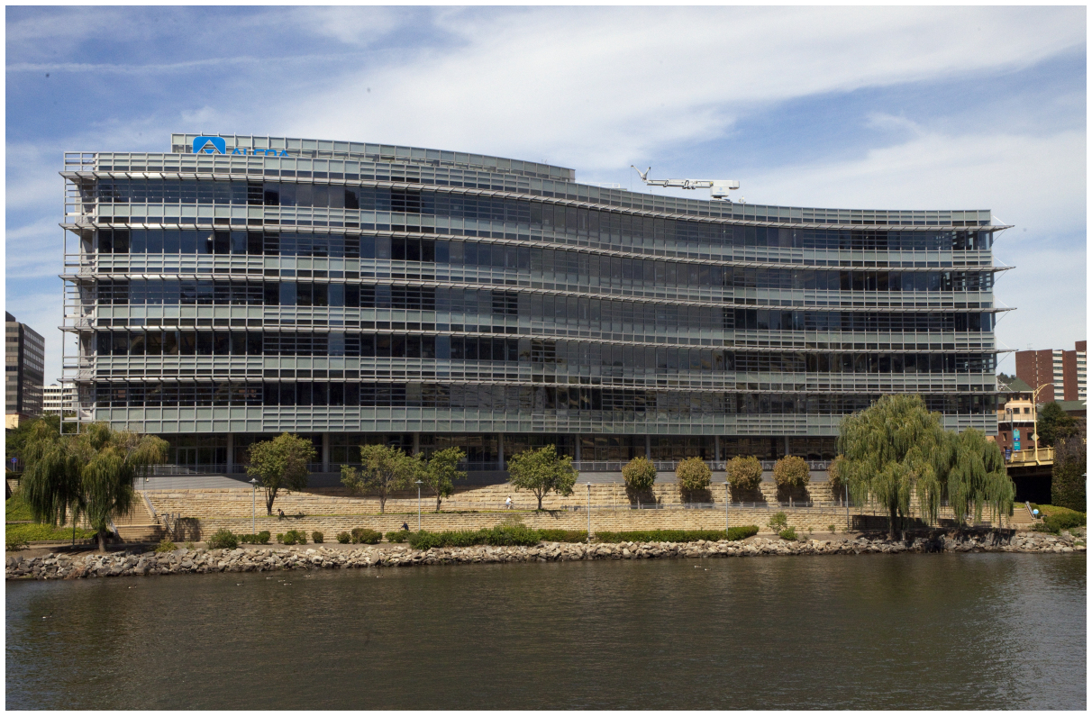
To motivate the discussion let us consider the Alcoa building, illustrated in this figure. Although three of the sides of the building shape are planar, the fourth one is a curvilinear surface. To simplify, we begin by considering that this curvilinear surface has a sinusoidal shape.

The Alcoa building, in Pittsburgh. Photograph by Roy Winkelman, from https://etc.usf.edu/clippix/picture/alcoa-building-in-pittsburgh-pennsylvania.html

As seen in section Extrusions, a sinusoid is determined by the following parameters: the amplitude \(a\), the angular frequency \(\omega\), i.e., the number of cycles per length unit, and the phase \(\phi\) of the curve in relation to the \(Y\) axis. With these parameters, the sinusoid equation has the form:

\[y(x) = a \sin(\omega x + \phi)\]

As also previously mentioned, the translation of the sinusoid equation to Julia is as follows:

sinusoid(a, omega, phi, x) = a*sin(omega*x+phi)

To calculate the points of a sinusoid we can use the aforementioned function sinusoid_points that computes an array of coordinates \((x,y)\) corresponding to the evolution of a sinusoid between the limits of a range \([x_0, x_1]\), with an increment \(\Delta_x\);

sinusoid_points(p, a, omega, phi, x0, x1, dx) =

if x0 > x1

[]

else

[p+vxy(x0, sinusoid(a, omega, phi, x0)),

sinusoid_points(p, a, omega, phi, x0+dx, x1, dx)...]

end

The previous function generates an array with points of the facade. In order to model the rest of the building, we need to join these points to form a curve, then we need to make a region with this curve and the lines that delimit the three rectilinear sides of the building, and finally we need to extrude this region. The length \(l\) of the building will be given by the distance between the two ends of the curved facade. The width \(w\) and height \(h\) will have to be parameters. Thus, we have:

building(points, w, h) =

let p0 = points[1],

p1 = points[end],

l = p1.x-p0.x

extrusion(surface(spline(points), line(p0, p0+vxy(0, w), p0+vxy(l, w), p1)),

h)

end

To visualize the capabilities of the previous function we can build several buildings using different values for the sinusoid’s parameters. In the following expressions we considered two rows of buildings, all with \(15\) meters long, \(10\) meters wide and \(20\) or \(30\) meters tall, depending on the row. This figure shows these buildings for different values of the parameters a, omega and phi:

building(sinusoid_points(xy(0, 0), 0.75, 0.5, 0, 0, 15, 0.4), 10, 20)

building(sinusoid_points(xy(25, 0), 0.55, 1.0, 0, 0, 15, 0.2), 10, 20)

building(sinusoid_points(xy(50, 0), 0.25, 2.0, 0, 0, 15, 0.1), 10, 20)

building(sinusoid_points(xy(0, 20), 0.95, 1.5, 0, 1, 15, 0.4), 10, 30)

building(sinusoid_points(xy(25, 20), 0.85, 0.2, 0, 0, 15, 0.2), 10, 30)

building(sinusoid_points(xy(50, 20), 0.35, 1.0, 0, 1, 15, 0.1), 10, 30)

Buildings containing sinusoidal facades with different values for the parameters.

Unfortunately, although the sinusoid_points function is very useful for modeling a multitude of different buildings with a sinusoidal facade, it is totally useless to model facades that follow other types of curves, such as parabolas, logarithmic, or exponential curves.

Naturally, nothing prevents us from defining other functions for modeling different facades. Let us imagine, for example, that we want a facade with the curvature of a parabola. The parabola with vertex at \((x_v,y_v)\) and focus point at \((x_v,y_v+d)\), with \(d\) being the distance from the vertex to the focus point, is defined by the following equation:

\[(x - x_v)^2 = 4d(y - y_v)\]

that is

\[y=\frac{(x - x_v)^2}{4d}+y_v\]

In Julia, this function is defined as:

parabola(xv, yv, d, x) = (x-xv)^2/(4*d)+yv

In order to generate the parabola’s points, we once again have to iterate over a range \([x_0, x_1]\) with a certain increment \(\Delta_x\):

parabola_points(p, xv, yv, d, x0, x1, dx) =

if x0 > x1

[]

else

[p+vxy(x0, parabola(xv, yv, d, x0)),

parabola_points(p, xv, yv, d, x0+dx, x1, dx)...]

end

The following expressions test this function with different values of the various parameters, generating the buildings represented in this figure:

building(parabola_points(xy(0, 0), 10, 0, 5, 0, 15, 0.5), 10, 20)

building(parabola_points(xy(25, 0), 5, 0, 3, 0, 15, 0.2), 10, 20)

building(parabola_points(xy(50, 0), 7, 1, -2, 0, 15, 0.1), 10, 20)

building(parabola_points(xy(0, 20), 8, 0, 2, 0, 15, 0.4), 10, 30)

building(parabola_points(xy(25, 20), 6, -2, 3, 0, 15, 0.2), 10, 30)

building(parabola_points(xy(50, 20), 5, 0, 6, 0, 15, 0.1), 10, 30)

Buildings containing parabolic facades with different parameters.

Once more, the parametrization of the function parabola_points allows us to generate an infinity of buildings containing facades with the curvature of a parabola, but these buildings will always be different from those that we can create with the sinusoid_points function. Although the modeling process used is absolutely identical in both cases, the base functions - sinusoid vs parabola - will always produce different curves.

Clearly, if we want to create buildings with a curved facade determined by a function \(f(x)\) that is neither a sinusoid nor a parabola, we cannot employ the previous functions. First, we will need to define the function f that implements that curve and, second, we will need to define the f_points function that generates the points of f in an interval. This second part seems overly repetitive and, indeed, it is. We simply have to observe the sinusoid_points and parabola_points functions to conclude that they are very similar to each other. Logically, the same will happen with the new f_points function.

This repetition leads us to consider the possibility of abstracting the process so that we are not obliged to repeat definitions that only vary in small details. By comparing the definitions of the functions sinusoid_points and parabola_points, if becomes clear that the only difference lies in the function that is invoked: sinusoid in the first case and parabola in the second case.

When two functions differ only in a name they use internally, it is always possible to define a third function that generalizes them, by simply transforming that name into an additional parameter. Suppose then that we make the following definition, where f is that additional parameter:

function_points(p, f, alpha, beta, gamma, x0, x1, dx) =

if x0 > x1

[]

else

[p+vxy(x0, f(alpha, beta, gamma, x0)),

function_points(p, f, alpha, beta, gamma, x0+dx, x1, dx)...]

end

The innovative look of the function_points function lies in the fact that it receives a function as an argument, a function which will be associated to the parameter f. When, in the body of the function_points function, a call is made of the f function, we are, actually, calling the function that has been passed as argument to the f parameter.

Thus, the expression

sinusoid_points(p, a, omega, phi, 0, lx, dx)

is absolutely identical to

function_points(p, sinusoid, a, omega, phi, 0, lx, dx)

Similarly, the expression

parabola_points(p, xv, yv, d, 0, lx, dx)

is absolutely identical to

function_points(p, parabola, xv, yv, d, 0, lx, dx)

More important than the fact that we can dismiss the sinusoid_points and parabola_points functions is the fact that, now, we can model buildings that contain facades following any other curve we want. For example, the function that describes the damped oscillatory motion has the definition:

\[y=ae^{-bx}\sin(cx)\]

or, in Julia:

damped_oscillation(a, b, c, x) = a*exp(-(b*x))*sin(c*x)

Using the function_points function, it is now easy to define a building that contains facades following the damped oscillatory motion. For example, the following expression produces, as a result of its evaluation, the building presented in this figure.

building(function_points(xy(0, 0), damped_oscillation, -5, 0.1, 1, 0, 40, 0.4),          10,          20)

A building with a facade that follows the curve of the damped oscillatory motion.