6.6 Trusses
A truss is a structure composed of rigid bars joined together at nodes, typically forming triangular units. Being the triangle the only polygon intrinsically stable, the interconnected triangles allow trusses to be structurally stable structures. Despite their simplicity, different arrangements of these triangular elements allow for different types of trusses.
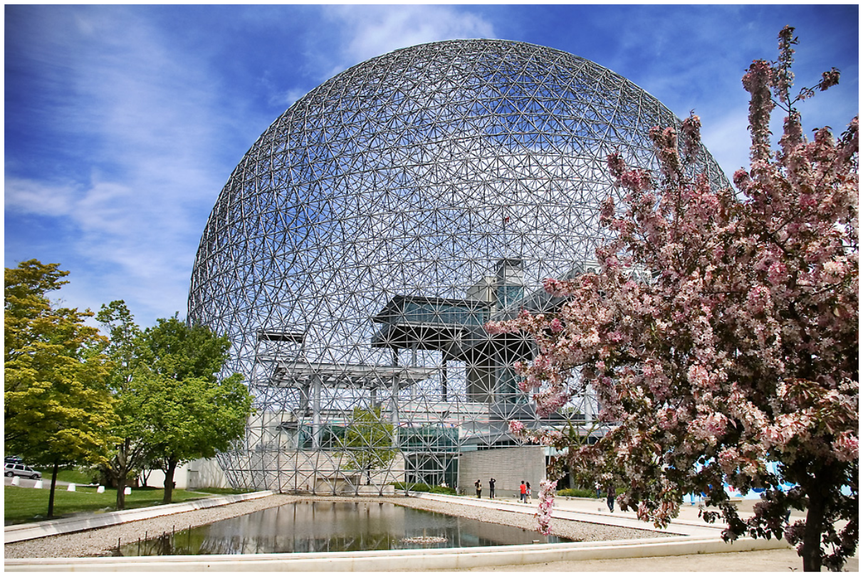
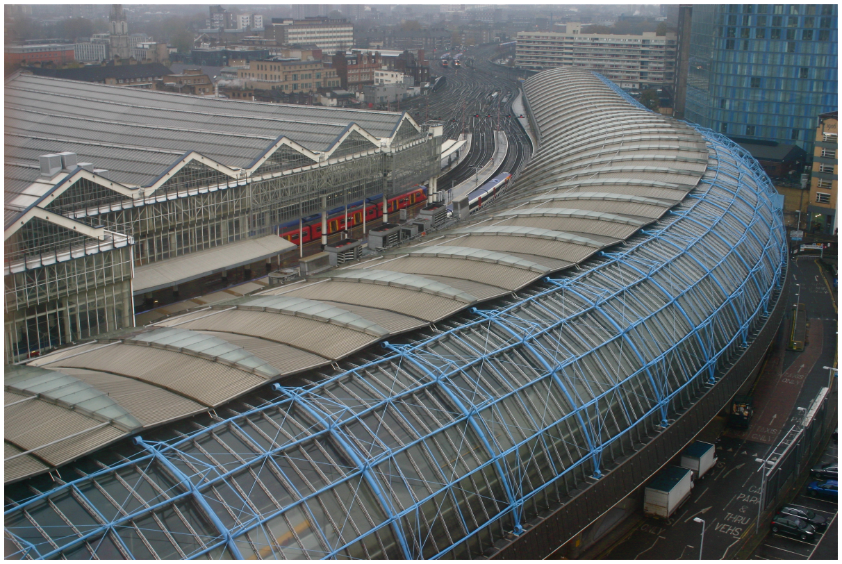
The use of trusses is known since ancient Greece, where they were used to support roofs. In the 16th century, Andrea Palladio illustrates bridges made of trusses in his The Four Books of Architecture. In the 19th century, with the extensive use of metal and the need to overcome increasing spans, different types of trusses were invented, varying in the different arrangements of vertical, horizontal, and diagonal bars. These types were frequently named after their inventors, e.g., Pratt truss, Howe truss, Town truss, and Warren truss. In the last decades, trusses began to be intensively used as an artistic element or for the construction of elaborate surfaces. Famous examples include the Buckminster Fuller’s geodesic dome originally constructed for the Universal Exposition of 1967, illustrated in this figure, and the banana-shaped trusses by Nicholas Grimshaw for the Waterloo terminal, visible in this figure.
The Buckminster Fuller’s geodesic dome. Photograph by Glen Fraser.
Banana-shaped trusses for the Waterloo terminal, by Nicholas Grimshaw. Photograph by Thomas Hayes.
Trusses have a set of properties that make them particularly interesting from an architectural point of view:
It is possible to build very large trusses from relatively small elements, which facilitates production, transportation, and construction;
Provided that the weight is applied only on the trusses’ nodes, the bars are only subject to axial forces, allowing structural forms of great efficiency;
As the basic elements are bars and nodes, it is easy to adapt its dimensions to the expected loads, allowing great flexibility.
6.6.1 Modeling Trusses
In order to algorithmically model a truss, we will start by studying the case of a three-dimensional truss composed by half-octahedrons, where each half-octahedron is called a module. This type of truss is also called a space frame. Other types of trusses can be derived from this one, including the bi-dimensional case known as planar truss.
This figure presents a scheme of a truss. Although the nodes are equally spaced along parallel lines, that is not a requirement, as visible in the truss illustrated in this figure.
Trusses composed by identical triangular elements.

Trusses composed by non-identical triangular elements.

To create a truss, we will start by considering three arbitrary sequences of points \((a_i, b_i, c_i)\) that define the location of the truss nodes. From these sequences we can establish the connections between pairs of nodes. This figure illustrates the connection scheme of three sequences of points \((a_0,a_1, a_2)\), \((b_0, b_1)\) and \((c_0, c_1, c_2)\). Note that the intermediate sequence \(b_i\) has one less element than the \(a_i\) and \(c_i\) sequences.
Bar connection scheme of a simple truss.

For the truss construction, we need to find a process that, from the arrays of points \(a_i\), \(b_i\) and \(c_i\), not only creates the corresponding nodes for the various points, but also interconnects them in the correct way. We will first focus on the creation of the nodes. Given a sequence of points \(p_i\), we need to create a truss node on each one. This can be done in two different ways. The first one is based on the use of recursion:
truss_nodes(ps) =
if ps == []
nothing
else
truss_node(ps[1])
truss_nodes(ps[2:end])
end
The second one uses the for control structure provided by the Julia language:
truss_nodes(ps) =
for p in ps
truss_node(p)
end
The truss_node function (note the use of the singular, instead of the plural used in the truss_nodes function) receives the coordinates of a point and creates the three-dimensional model of a truss node centered in that point. One simple approach for this function is to create a sphere to which the bars will be then connected.
Using the truss_nodes function, we can start idealizing the function that builds a complete truss from the arrays of points as, bs and cs:
truss(as, bs, cs) =
begin
truss_nodes(as)
truss_nodes(bs)
truss_nodes(cs)
...
end
Next, let us establish the bars between the nodes. From analyzing this figure, we realize we have one connection between each of the following pairs: \(a_i\) and \(c_i\), \(a_i\) and \(b_i\), \(b_i\) and \(c_i\), \(b_i\) and \(a_{i+1}\), \(b_i\) and \(c_{i+1}\), \(a_i\) and \(a_{i+1}\), \(b_i\) and \(b_{i+1}\) and, finally, \(c_i\) and \(c_{i+1}\). Admitting that the truss_bar function creates the three-dimensional model of each bar (for example, a cylindrical or prismatic bar), we start by defining a function denominated truss_bars (note the plural) that, given two arrays of points ps and qs, creates the connection bars along successive pairs of points. To create a bar, the function needs one element from the array ps and another from the array qs, which implies that the function must end as soon as one of these arrays is empty. Therefore, the definition is:
truss_bars(ps, qs) =
if ps == [] || qs == []
nothing
else
truss_bar(ps[1], qs[1])
truss_bars(ps[2:end], qs[2:end])
end
Similarly to the function truss_nodes, this particular kind of recursion can be done with a for operation but, this time, working with pairs of elements. These pairs can be produced with the zip function that, from two arrays, produces an array of pairs.
truss_bars(ps, qs) =
for (p, q) in zip(ps, qs)
truss_bar(p, q)
end
Continuing with the definition of the truss function, we need to evaluate the expression truss_bars(as, cs) to connect each \(a_i\) node to its corresponding \(c_i\) node. The same can be said for connecting each \(a_i\) node to its corresponding \(b_i\) node, and each \(b_i\) node to its corresponding \(c_i\) node. Thus, we have:
truss(as, bs, cs) =
begin
truss_nodes(as)
truss_nodes(bs)
truss_nodes(cs)
truss_bars(as, cs)
truss_bars(as, bs)
truss_bars(bs, cs)
...
end
To connect the \(b_i\) nodes to the \(a_{i+1}\) nodes, we can simply remove the first node from the array as and establish the connections as before. The same can be done to connect each \(b_i\) to each \(c_{i+1}\), and, finally, to connect each \(a_i\) to \(a_{i+1}\), each \(b_i\) to \(b_{i+1}\), and each \(c_i\) to \(c_{i+1}\). The complete truss function is the following:
truss(as, bs, cs) =
begin
truss_nodes(as)
truss_nodes(bs)
truss_nodes(cs)
truss_bars(as, cs)
truss_bars(as, bs)
truss_bars(bs, cs)
truss_bars(bs, as[2:end])
truss_bars(bs, cs[2:end])
truss_bars(as, as[2:end])
truss_bars(bs, bs[2:end])
truss_bars(cs, cs[2:end])
end
Lastly, all we need to do is to define the truss_node and the truss_bar functions. For now, we will consider that a truss node is a sphere and a truss bar is a cylinder. Both the spheres and cylinders radii will be determined by global variables, so that we can easily change their value. Thus, we have:
truss_node_radius = 0.1
truss_node(p) = sphere(p, truss_node_radius)
truss_bar_radius = 0.03
truss_bar(p0, p1) = cylinder(p0, truss_bar_radius, p1)
Having these functions, we can create a large variety of trusses. This figure shows a truss drawn from the expression:
truss([xyz(0, -1, 0),
xyz(1, -1.1, 0),
xyz(2, -1.4, 0),
xyz(3, -1.6, 0),
xyz(4, -1.5, 0),
xyz(5, -1.3, 0),
xyz(6, -1.1, 0),
xyz(7, -1, 0)],
[xyz(0.5, 0, 0.5),
xyz(1.5, 0, 1),
xyz(2.5, 0, 1.5),
xyz(3.5, 0, 2),
xyz(4.5, 0, 1.5),
xyz(5.5, 0, 1.1),
xyz(6.5, 0, 0.8)],
[xyz(0, 1, 0),
xyz(1, 1.1, 0),
xyz(2, 1.4, 0),
xyz(3, 1.6, 0),
xyz(4, 1.5, 0),
xyz(5, 1.3, 0),
xyz(6, 1.1, 0),
xyz(7, 1, 0)])
Truss build from a set of specified points.

6.6.1.1 Question 105
Define the straight_truss function, capable of building any of the trusses shown in the following image.

To simplify, consider that these trusses develop along the \(X\) axis. The straight_truss function should receive the initial point of the truss, the height and length of the truss and the number of nodes of the lateral rows. With these values, the function should be defined upon the truss function, which receives three arrays of coordinates as arguments. As an example, consider that the three trusses presented in the previous image resulted from the evaluation of the following expressions:
straight_truss(xyz(0, 0, 0), 1.0, 1.0, 20)
straight_truss(xyz(0, 5, 0), 2.0, 1.0, 20)
straight_truss(xyz(0, 10, 0), 1.0, 2.0, 10)
Suggestion: define a linear_positions function that, given an initial point \(P\), a separation between points \(l\), and a number of points \(n\), returns an array with the coordinates of \(n\) points arranged along the \(X\) axis.
6.6.1.2 Question 106
The total cost of a truss highly depends on the number of different lengths that the bars may have: the smaller the number, the greater economies of scale can be obtained and, consequently, the cheaper the truss will be. The ideal scenario is when all bars have the same length.
Given the following scheme, determine the height \(h\) of the truss in terms of the length \(l\) of the module, so that all the bars have the same length.

Then, define the truss_equilateral function that builds a truss with all the bars having the same length, and oriented along the \(X\) axis. The function should receive the truss initial point, its length and the number of nodes of the lateral rows.
6.6.1.3 Question 107
Consider the following scheme of a planar truss:

Define a planar_truss function that receives two arrays as arguments, one containing the points from \(a_0\) to \(a_n\), and the other containing the points from \(b_0\) to \(b_{n-1}\). The function should create nodes in those points and bars joining them. As a suggestion, consider the previously defined functions truss_nodes, which receives one array of positions as argument, and truss_bars, which receives two arrays of positions as arguments.
Test the function with the following expression:
planar_truss(linear_positions(xyz(0, 0, 0), 2.0, 20),
linear_positions(xyz(1, 0, 1), 2.0, 19))
6.6.1.4 Question 108
Consider the T-shaped truss represented in the following figure:

Define a t_shaped_truss function that, given three arrays containing, respectively, the points from \(a_0\) to \(a_n\), \(b_0\) to \(b_{n-1}\), and \(c_0\) to \(c_n\), creates nodes at those points and bars joining them. Again, consider the previously defined functions truss_nodes, which receives one array of positions as argument, and truss_bars, which receives two arrays of positions as arguments.
6.6.2 Creating Positions
As we saw in the previous section, it is possible to define a process of creating a truss from arrays containing its node positions. Although these arrays can be specified manually, this approach is only viable for very small trusses. Being the truss a structure capable of covering very large spans, the number of truss nodes is, in most cases, too large for us to manually produce the corresponding array of positions. To solve this problem, we must automate the creation of these arrays, taking into account the desired geometry of the truss.
As an example, we will now create a truss with the shape of an arc, in which the node sequences \(a_i\), \(b_i\) and \(c_i\) form circumference arcs. This figure shows one such truss, defined by the circumference arcs of radius \(r_ac\) and \(r_b\). The truss nodes are distributed in three arcs: two lateral arcs (containing the \(a_i\) and \(c_i\) node sequences) and one intermediate arc (containing the \(b_i\) node sequence).
To make the truss uniform, the nodes are equally spaced along the arc: the angle \(\Delta_\psi\) corresponds to that spacing, and it is calculated by dividing the arc angle amplitude by the number of nodes required. As the intermediate arc always has one less node than the lateral arcs, we need to divide the \(\Delta_\psi\) angle by the two extremities of the intermediate arc, in order to center these arc’s nodes in between the nodes of the lateral arcs, as it is visible in this figure.
Front view of a truss in shape of a circular arc.

Since the arc is circular, the simplest way of calculating the node positions is using spherical coordinates \((\rho, \phi,\psi)\). Therefore, the initial and final angles of the arcs should be measured relatively to the \(Z\) axis, as visible in this figure. To produce the coordinates of each arc nodes, we will define a function that takes the center \(P\) of the arc, the radius \(r\) of that arc, the angle \(\phi\), the initial \(\psi_0\) and final \(\psi_1\) angles and finally, the angle increment \(\Delta_\psi\). Thus, we have:
arc_positions(p, r, phi, psi0, psi1, dpsi) =
if psi0 > psi1
[]
else
[p+vsph(r, phi, psi0), arc_positions(p, r, phi, psi0+dpsi, psi1, dpsi)...]
end
To build the arc truss, we can now define a function that creates three of the previous arc_positions. To this end, the function receives the center \(P\) of the intermediate arc, the radius \(r_{ac}\) of the lateral arcs, the radius \(r_b\) of the intermediate arc, the angle \(\phi\), the initial angle \(\psi_0\) and final angle \(\psi_1\), the length \(l\) between the lateral arcs, and the number \(n\) of nodes of the lateral arcs. The function starts by calculating the angle increment \(\Delta_\psi=\frac{\psi_1-\psi_0}{n}\), and then calls the truss function with the appropriate parameters:
arc_truss(p, rac, rb, phi, psi0, psi1, l, n) =
let dpsi = (psi1-psi0)/n
truss(arc_positions(p+vpol(l/2.0, phi+pi/2), rac, phi, psi0, psi1, dpsi),
arc_positions(p, rb, phi, psi0+dpsi/2.0, psi1-dpsi/2.0, dpsi),
arc_positions(p+vpol(l/2.0, phi-pi/2), rac, phi, psi0, psi1, dpsi))
end
This figure shows the trusses built with the expressions:
arc_truss(xyz(0, 0, 0), 10, 9, 0, -pi/2, pi/2, 1.0, 20)
arc_truss(xyz(0, 5, 0), 8, 9, 0, -pi/3, pi/3, 2.0, 20)
Arc trusses created with different parameters.

6.6.2.1 Question 111
Consider the construction of vaults supported on trusses radially distributed, such as the one displayed in the following image:

This vault is composed by a given number of circular arc trusses. The length \(l\) of each truss and the initial angle \(\psi_0\) with which each truss starts are such that the trusses top nodes are coincident in pairs and are arranged along a circle of radius \(r\), as shown in the following scheme:

Define the truss_vault function that builds a vault of trusses from the vault center point \(P\), the radius \(r_{ac}\) of the lateral arcs of each truss, the radius \(r_b\) of the intermediate arc of each truss, the radius \(r\) of the top nodes of the trusses, the number \(n\) of nodes in the lateral arcs of each truss and, finally, the number \(n_\phi\) of trusses.
As an example, consider the figure below, produced by the evaluation of the following expressions:
truss_vault(xyz(0, 0, 0), 10, 9, 2.0, 10, 3)
truss_vault(xyz(25, 0, 0), 10, 9, 2.0, 10, 6)
truss_vault(xyz(50, 0, 0), 10, 9, 2.0, 10, 9)

6.6.2.2 Question 109
Consider the creation of a ladder identical to the one shown on the following figure:

Note that the ladder is a (very) simplified version of a truss composed only by two sequences of nodes. Define the ladder function that receives two arrays of points and creates nodes at those points and bars joining them. Again, consider the previously defined functions truss_nodes, which receives one array of positions as argument, and truss_bars, which receives two arrays of positions as arguments.
6.6.2.3 Question 110
Define a function capable of representing the DNA double helix, as shown in the following image:

The function should receive the position of the DNA base center, the radius of the DNA helix, the angular difference between the nodes, the height difference between the nodes, and, finally, the number of nodes in each helix. The DNA double helices represented in the previous image were created by the following expressions:
dna(xyz(0, 0, 0), 1.0, pi/32, 0.5, 20)
dna(xyz(4, 0, 0), 1.0, pi/16, 0.25, 40)
dna(xyz(8, 0, 0), 1.0, pi/8, 0.125, 80)
6.6.3 Space Trusses
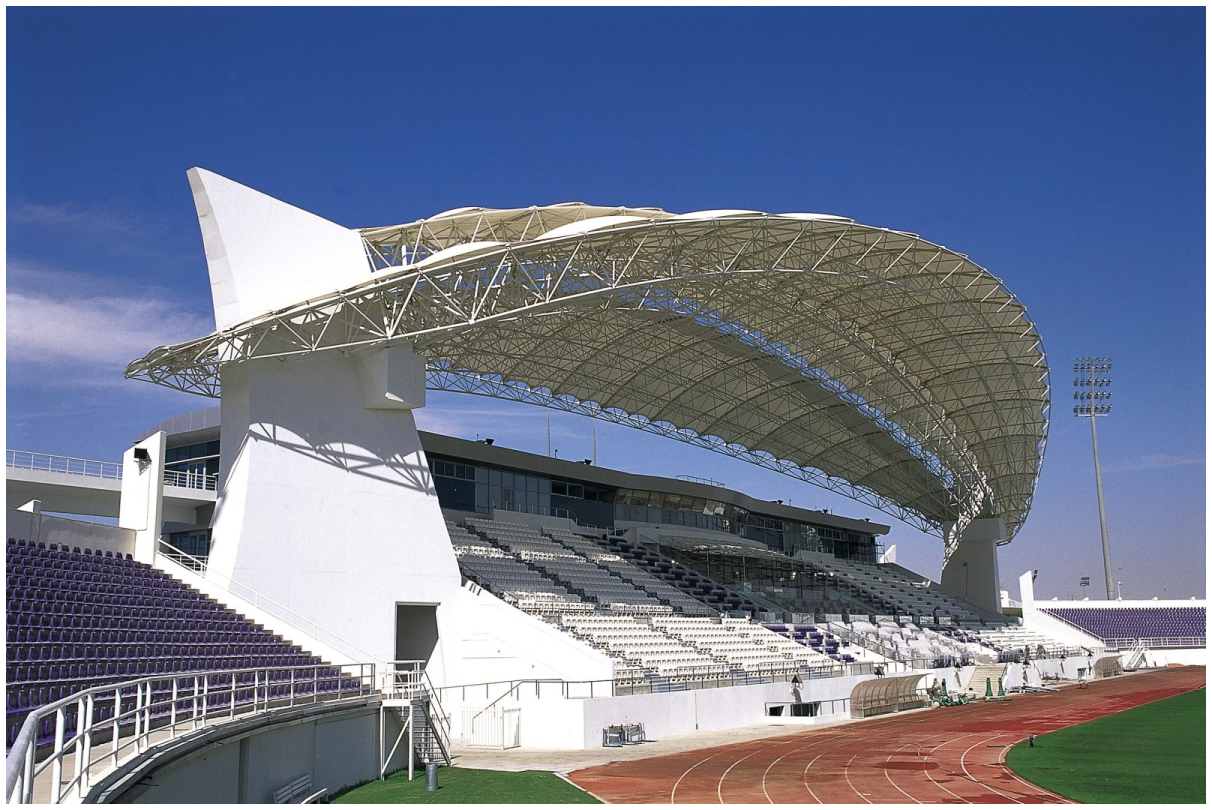
We have seen how it is possible to define simple trusses from three arrays, each containing the nodes’ coordinates to which the bars are connected. By connecting various of these trusses with each other, we can create an even bigger structure: the space truss. This figure shows an example where three space trusses are visible.
Space trusses in the Khalifa bin Zayed Stadium in Al Ain, United Arab Emirates. Photograph by Klaus Knebel.
In order to define an algorithm that generates space trusses, we need to consider that the trusses are interconnected so that each truss shares a set of nodes and bars with the adjacent truss. This is visible in this figure, which illustrates a space truss scheme. This means that a space truss composed by two simple interconnected trusses contains only five arrays of coordinates, instead of six. In the general case, a space truss formed by \(n\) simple trusses will be defined by \(2n+1\) arrays of points.
Bar connection scheme of a space truss.

The function that creates a space truss follows the same logic of the function that creates a simple truss but, instead of operating with only three arrays, it operates with an array of arrays, where each array represents a row of truss nodes. Each node is now represented by two indexes, where the first indicates the truss where it belongs and the second its position within the truss. Moreover, the elements \(c_{i,j}\) of a truss are also the elements \(a_{i+1,j}\) of the following truss. This means that the array of arrays has the following format:
\(\begin{align*} [&[a_{0,0}\quad a_{0,1}\quad a_{0,2}\quad \ldots{}\quad a_{0,n-1}\quad a_{0,n}]\\ &[b_{0,0}\quad b_{0,1}\quad b_{0,2}\quad \ldots{}\quad b_{0,n-1}]\\ &[a_{1,0}\quad a_{1,1}\quad a_{1,2}\quad \ldots{}\quad a_{1,n-1}\quad a_{1,n}]\\ &\ldots{}\\ &[c_{m,0}\quad c_{m,1}\quad c_{m,2}\quad \ldots{}\quad c_{m,n-1}\quad c_{m,n}]] \end{align*}\)
Note that the function will have to receive an odd number of node rows. The function processes two arrays at a time (the \(a_{i,j}\) row of nodes and the \(b_{i,j}\) row of nodes). In the final truss (when only three of rows of nodes remain), the final row of \(c_{m,j}\) nodes is generated.
There is, however, an additional difficulty: for the space truss to have transversal rigidity, it is necessary to connect the central nodes of the various trusses with each other, i.e., to connect each \(b_{i,j}\) node to the \(b_{i+1,j}\) node. The entire process is implemented by the following function:
space_truss(ptss) =
let as = ptss[1]
bs = ptss[2]
cs = ptss[3]
truss_nodes(as)
truss_nodes(bs)
truss_bars(as, cs)
truss_bars(as, bs)
truss_bars(bs, cs)
truss_bars(bs, as[2:end])
truss_bars(bs, cs[2:end])
truss_bars(as, as[2:end])
truss_bars(bs, bs[2:end])
if length(ptss) == 3 # no nodes left?
truss_nodes(cs)
truss_bars(cs, cs[2:end])
else
space_truss(ptss[3:end])
truss_bars(bs, ptss[4])
end
end
6.6.3.1 Question 112
In reality, a simple truss is a particular case of a space truss. Redefine the truss function so that it uses the space_truss function.
Now that we know how to build space trusses from an array of arrays of positions, we can think of mechanisms to generate this array of arrays. A simple example is the horizontal space truss presented in this figure.
A horizontal space truss composed of eight simple trusses with ten pyramids each.

To generate the coordinates of the nodes, we can define a function that, based on the number of desired nodes and on the length of the pyramid base, generates the nodes along one of the dimensions, for example, the \(X\) dimension:
linear_positions(p, l, n) =
if n == 0
[]
else
[p, linear_positions(p+vx(l), l, n-1)...]
end
Next, we only have to define a function that iterates the previous one along the \(Y\) dimension, generating successive \(a_{i}\) and \(b_{i}\) node rows until the end, when we have to generate an extra \(a_{i}\) row. In this process, it is necessary to take into account that the \(b_{i}\) rows have one less node then the \(a_{i}\) rows. Based on these considerations, we can write:
horizontal_truss_positions(p, h, l, n, m) =
if m == 0
[linear_positions(p, l, n)]
else
[linear_positions(p, l, n),
linear_positions(p+vxyz(l/2, l/2, h), l, n-1),
horizontal_truss_positions(p+vy(l), h, l, n, m-1)...]
end
We can now combine the array of arrays of positions created by the previous function with the one that creates a space truss. As an example, the following expression creates the truss shown in this figure:
space_truss(horizontal_truss_positions(xyz(0, 0, 0), 1, 1, 9, 10))
6.6.4 Exercises 32
6.6.4.1 Question 113
Consider the creation of a random space truss. In this truss the nodes are positioned at a random distance from the correspondent nodes of a horizontal space truss. An example is shown in the figure below, in which the bars that join the \(a_i\), \(b_i\), and \(c_i\) nodes where highlighted to facilitate visualization.

Define the function random_truss_positions that, in addition to the horizontal_truss_positions function parameters, receives the maximum distance \(r\) that each node from the random truss can be placed relatively to the correspondent node of the horizontal truss. As an example, consider the truss presented in the previous figure, which was created by the evaluation of the following expression:
space_truss(random_truss_positions(xyz(0, 0, 0), 1, 1, 9, 10, 0.2))
6.6.4.2 Question 114
Consider the creation of an arched space truss, like the one presented in the following image. Define the arched_space_truss function that, besides the parameters of the arc_truss function (previously defined), has an additional parameter indicating the number of simple trusses that it contains. As an example, consider the truss shown in the following image, which was created by the expression:
arched_space_truss(xyz(0, 0, 0), 10, 9, 0, -pi/3, pi/3, 1.0, 20, 10)

6.6.4.3 Question 115
Consider the truss illustrated in the image below:

This truss is similar to the arched space truss, except that the radii rac and rb of the exterior and interior arcs follow a sinusoid of amplitude \(\Delta_r\), varying from an initial value \(\alpha_0\) to a final value \(\alpha_1\), in increments of \(\Delta_\alpha\).
Define the wave_truss function that, given the same parameters as the arched_space_truss function plus the parameters \(\alpha_0\), \(\alpha_1\), \(\Delta_\alpha\) and \(\Delta_r\), creates this type of truss. As an example, consider the previous figure, which was created by the following expression:
wave_truss(xyz(0, 0, 0), 10, 9, 0, -pi/3, pi/3, 1.0, 20, 32, 0, 4*pi, pi/8, 1)