6.4 Polygons

Arrays are particularly useful to represent abstract geometrical entities, i.e., entities about which we are only interested in knowing certain properties, such as their position. In that case, we can use an array of positions, i.e., an array in which the elements represent positions in space.

As an example, imagine we want to represent a polygon. By definition, a polygon is a plane figure bounded by a closed path composed by a sequence of line segments. Each line segment is an edge (or side) of the polygon. Each point where two line segments meet is a vertex of the polygon.

Based on this definition, it is easy to infer that one of the simplest ways to represent a polygon is through a sequence of positions indicating the positions of the vertices by the order we should connect them, admitting the last element is connected to the first one. It is precisely this sequence of arguments that we provide in the following example of the Khepri’s polygon function (see the Bi-dimensional Drawing section):

polygon(xy(-2, -1), xy(0, 2), xy(2, -1))

polygon(xy(-2, 1), xy(0, -2), xy(2, 1))

The result of evaluating these expressions is shown in this figure.

Two overlapping polygons.

Now, let us suppose that, rather than explicitly indicate each vertex position, we want a function to produce that same sequence of positions. For this, the use of arrays constitutes a valuable help, since they allow the representation of sequences. Moreover, many of the geometric functions, such as line and polygon, also accept an array as argument. In fact, this figure can be reproduced by the following expressions:

polygon([xy(-2, -1), xy(0, 2), xy(2, -1)])

polygon([xy(-2, 1), xy(0, -2), xy(2, 1)])

In the same way that a triangle can be represented by an array with three vertices, a quadrilateral can be represented by an array with four vertices, an octagon can be represented by an array with eight vertices, a triacontakaihenagon can be represented by an array with thirty-one vertices, and so on. In the next sections we will focus on how to create these arrays.

6.4.1 Regular Stars

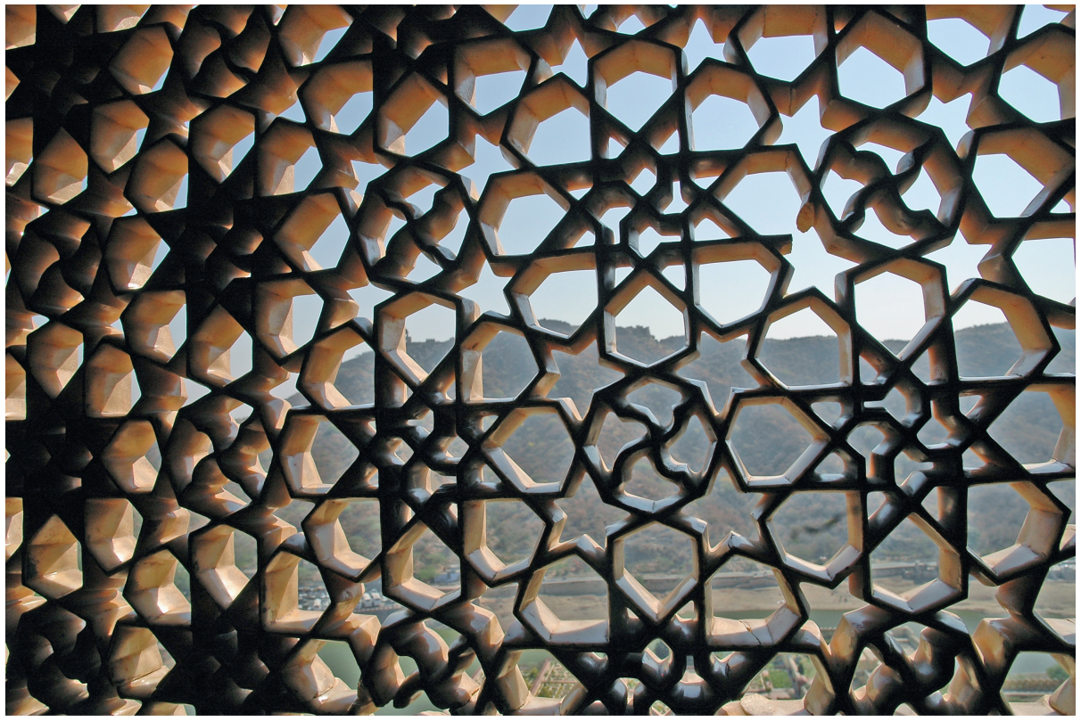
A regular star is a self-intersecting polygon with equal side lengths and equal vertex angles. The famous pentagram, or five point star, is a star polygon that has been used with symbolic, magical, or decorative purposes since Babylonian times. The pentagram was the symbol of mathematical perfection for the Pythagoreans, the symbol of the supremacy of the spirit over the four elements of matter for the occultists, and the symbol of the Five Holy Wounds of Christ for the Christians. The pentagram was also associated with the proportions of the human body, and has been used by the Freemasonry and, when inverted, by Satanic cults. This figure illustrates the use of the pentagram (as well as the octagram, the octagon and the hexagon) as part of a structural and decorative window made of stone.

Variations of star polygons in a window of the Amber Fort, located in the district of Jaipur, India. Photograph by David Emmett Cooley.

Apart from the symbolic connotations, the pentagram is, first of all, a polygon. For this reason, it can be drawn by the polygon function, as long as we produce an array with the positions of its vertices. To that end, we will now focus on this figure, where we see that the five pentagram vertices divide the circle into 5 parts with arcs measuring \(\frac{2\pi}{5}\) each. From the pentagram’s center, its top vertex makes an angle of \(\frac{\pi}{2}\) with the \(X\) axis. This top vertex must then be connected, not with the next vertex, but with the one immediately after it, i.e., the one corresponding to a rotation of two arcs or \(\frac{2\cdot 2\pi}{5}=\frac{4}{5}\pi\). We can now define the pentagram_vertices function that creates the array of vertices of the pentagram:

pentagram_vertices(p, r) =   [p+vpol(r, pi/2+0*4/5*pi),    p+vpol(r, pi/2+1*4/5*pi),    p+vpol(r, pi/2+2*4/5*pi),    p+vpol(r, pi/2+3*4/5*pi),    p+vpol(r, pi/2+4*4/5*pi)]

To generate the pentagram visible in this figure, we just to compute, for example:

polygon(pentagram_vertices(xy(0, 0), 2))

Creation of a pentagram.

It is clear that the pentagram_vertices function contains a lot of repetitive code, so we need to find a more structured way of generating the pentagram vertices. As before, we could use recursion but, when the goal is the generation of an array of elements where each element can be described by a formula, as it happens with the pentagram_vertices function, it is possible to use a simpler approach, inspired on the syntax used in mathematics to specify array comprehensions. Using array comprehensions, the pentagram_vertices can be written as:

pentagram_vertices(p, r) =

[p + vpol(r, pi/2 + i*4/5*pi)

for i in [0, 1, 2, 3, 4]]

In the previous definition, the array of positions is created from a calculation involving the variable \(i\), in which \(i\) successively takes on each value in the array [0, 1, 2, 3, 4]. We can further simplify the function by using ranges. As previously discussed, a range allows us to represent an array of consecutive numbers as a pair containing the first and last number:

pentagram_vertices(p, r) =

[p + vpol(r, pi/2 + i*4/5*pi)

for i in 0:4]

Although the pentagram_vertices function is only capable of producing the vertices of a pentagram, it can be generalized to a function that can handle as many vertices as we want.

To generalize the pentagram_vertices function, we just need to consider the constants being used in the function as parameters, so that they can be varied. The initial angle \(pi/2\) becomes the parameter \(\phi\), the angle increment \(4/5\pi\) becomes \(\Delta\phi\), and the number of vertices becomes \(n\). This leads us to a general definition that we will call n-grams, which is capable of producing the vertices of pentagrams, hexagrams, heptagrams, and so on:

ngram_vertices(p, r, phi, dphi, n) =

[p + vpol(r, phi + i*dphi)

for i in 0:n-1]

We can now rewrite the pentagram_vertices function as a particular case of the ngram_vertices function, using pi/2 as the value of the initial angle phi, 4/5*pi as the value of the angle increment dphi and, finally, 5 as the number of vertices n:

pentagram_vertices(p, r) =

ngram_vertices(p, r, pi/2, 4/5*pi, 5)

The general case of a pentagram is the regular star polygon. In mathematics, a regular star is represented by the Schläfli symbol Ludwig Schläfli was a Swiss mathematician and geometer who made important contributions, especially to multidimensional geometry. \[\left\{\frac{v}{a}\right\}\], where \(v\) is the number of vertices and \(a\) is the number of arcs that separate a vertex from the vertex to which it connects. In this notation, the pentagram is written as \(\left\{\frac{5}{2}\right\}\).

In order to draw regular stars, we will write a function which, given the center of the star, the radius of the circumscribed circle, the number of vertices \(v\) (which we will call n_vertices) and the number of separation arcs \(a\) (which we will call n_arcs), calculates the value of the angle increment dphi. This angle will be, logically, \(\Delta\phi=a\frac{2\pi}{v}\). As in the pentagram, we will consider an initial angle of \(\phi=\frac{\pi}{2}\).

star_vertices(p, radius, n_vertices, n_arcs) =

ngram_vertices(p, radius, pi/2, n_arcs*2*pi/n_vertices, n_vertices)

Using the star_vertices function it is now trivial to generate the vertices of any regular star. This figure presents a set of regular stars generated by the following expressions:

polygon(star_vertices(xy(0, 0), 1, 5, 2))

polygon(star_vertices(xy(2, 0), 1, 7, 2))

polygon(star_vertices(xy(4, 0), 1, 7, 3))

polygon(star_vertices(xy(6, 0), 1, 8, 3))

Regular stars \(\left\{\frac{v}{a}\right\}\). From left to right: one pentagram (\(\left\{\frac{5}{2}\right\}\)), two heptagrams (\(\left\{\frac{7}{2}\right\}\) and \(\left\{\frac{7}{3}\right\}\)), and one octagram (\(\left\{\frac{8}{3}\right\}\)).

This figure shows a sequence of regular stars \(\left\{\frac{20}{r}\right\}\) with \(r\) varying between \(1\) and \(9\).

Regular stars \(\left\{\frac{p}{r}\right\}\) with \(p=20\) and \(r\) varying between \(1\) (on the left) and \(9\) (on the right).

It is very important to understand that the construction of stars is divided into two distinct parts. In the first part, we use the function star_vertices to produce the coordinates of the stars’ vertices in the order by which they must be connected. In the second part, we connect the vertices using the polygon function, which creates a graphical representation of the star. The transmission of information between these two functions is done using an array that is produced on one side and used on the other side.

The use of arrays to separate different processes is a fundamental strategy that will be repeatedly used to simplify our programs.

6.4.2 Regular Polygons

A regular polygon is a polygon with both equal side lengths and equal vertex angles. This figure illustrates examples of regular polygons. By simple observation, we can see that a regular polygon is a particularly case of a regular star in which there is only one arc between vertices.

Regular polygons, from left to right: an equilateral triangle, a square, a regular pentagon, a regular hexagon, a regular heptagon, a regular octagon, a regular enneagon and a regular decagon.

To create regular polygons, we can define a function called regular_polygon_vertices that generates an array of coordinates matching the vertices of a regular polygon with \(n\) sides, inscribed in a circle of radius \(r\) and center \(P\), and with an initial angle (between the first vertex and the \(X\) axis) \(\phi\). Being the regular polygon a particular case of a regular star, we only need to say that the number of arcs between the vertices is \(1\):

regular_polygon_vertices(n, p, r, phi) = star_vertices(p, r, n, 1)

Finally, we can combine the generation of vertices with their graphical use to create the corresponding polygon:

regular_polygon(n, p, r, phi) = polygon(regular_polygon_vertices(n, p, r, phi))

This figure shows a sequence of regular polygons.

Regular polygons, with the number of vertices ranging from \(3\) (on the left) to \(11\) (on the right).

Although we defined them here, the functions regular_polygon_vertices and regular_polygon are already predefined in Khepri.