ROSETTA

Contents:
• Part I - Random numbers
• Part II - Using random numbers to make choices
• Part III - Functions with state

We know by now that computer programs must be as clear as possible, without any kind of ambiguity. Computers do not possess imagination that is sometimes needed to interpret a particular solution to a problem so the programs we’ve written so far have had to be rigorous and rational. However, the design process in architecture often goes through phases of uncertainty where a great deal of experimentation is required. We don’t always know exactly what we want or maybe we do know but we still accept that there are many other solutions that are worth exploring before we make the final decision. Another situation where there may be some uncertainty during the design process is when we get inspiration from nature and try to mimic some of its aspects and patterns in our designs. These situations of uncertainty require some randomness, albeit a controlled randomness. If we want to design a building’s facade we may want to explore different geometric shapes for the openings, if we want to design a curtain wall we may want to test different way of dividing the glazing, if we want do divide an open space into smaller partitions we may want to test different sizes for them, etc. In these situations we already have a rough idea of what we want or the spectrum of possibilities we wish to test.

Thus far we have given specific values to the parameters in our functions but that needn’t be the case. We can very easily use a generator of random numbers to choose the parameters values for us. Racket provides the function random for this. The user provides a number n, either exact or inexact, and the random function will generate a pseudo-random number between zero and n-1. If n is exact then the generated number will also be exact and inexact if n is inexact. Let’s see some examples:

> (random 10)
6
> (random 10)
1
> (random 10)
9
> (random 10)
0
> (random 16.0)
9.358875830359233
> (random 16.0)
14.626080847636834
> (random 16.0)
12.540806232272091
> (random 16.0)
5.3303457970406605

We used the term pseudo-random number because the generated number is not entirely random. Based on an initial value provided by the user, also called a seed, the generator produces a series of apparently random numbers, each based on the previously generated one. Every the seed value is given the generator will always return the same generated number. This is particularly important for debugging. If a program has a bug but that program has a different behaviour each time it’s executed we may only encounter the bug on very rare occasions, making it very difficult or almost impossible to fix it. It is therefore important that we’re able to reproduce the conditions that lead to the bug happening so we can fix it.

Often we may not want to produce a random value between 0 and n-1 but rather between k and n-1. For that we can use Rosetta’s function random-range which receives as parameters the bottom and top limits:

> (random-range 10 20)
19
> (random-range 10 20)
12
> (random-range 10 20)
11
> (random-range 10 20)
14
> (random-range 10 20)
18
> (random-range 10 20)
12
> (random-range -6.0 0.0)
-5.106679664508756
> (random-range -6.0 0.0)
-3.965121398663671
> (random-range -6.0 0.0)
-5.7953473403096885

Now we can incorporate this generator in a function that creates geometry. If we create a square where one of its dimensions is generated randomly then each time we execute that function it will produce a different result every time.

> (rectangle (xy 0 0) 10 (random-range 10 30))
#<rectangle 0>
> (rectangle (xy 15 0) 10 (random-range 10 30))
#<rectangle 1>
> (rectangle (xy 30 0) 10 (random-range 10 30))
#<rectangle 2>
> (rectangle (xy 45 0) 10 (random-range 10 30))
#<rectangle 3>
> (rectangle (xy 60 0) 10 (random-range 10 30))
#<rectangle 4>

FIGURE 1 | A series of rectangles with a random height

When used along with recursion random numbers acquire a new very useful dimension. We can make so that each time the function is executed during the recursive process a new value is generated for a particular parameter or coordinate. If, for example, we wanted to populate a rectangular domain with a series of random point coordinates we could use the random-range to generate the coordinates and then recursively calculate a new random coordinate for the remaining points. If p is the rectangle insertion point, l and w are the rectangle dimensions and n is the number of points we wish to generate then our populate-2d function will be:

The bottom limits for the point coordinates are the x and y coordinates of p and the top limits are l and w, this way we are sure the generated points will be contained by the imaginary rectangle. We can now test the function but remember that the exactness of the generated coordinates depends on the exactness of the parameters l and w. If we invoke the function with l and w as exact numbers then there won’t be a lot of variability in our coordinates and we’ll most likely get a lot of coincidental points since every coordinate will get rounded to its integer equivalent. Just for the sake of showing this, both cases have been included in Figure 2, and because the function is just generating abstract data that we can’t see we have also included in the figure the rectangle boundary and a point with the corresponding coordinates to represent it. These are not included in our function though.

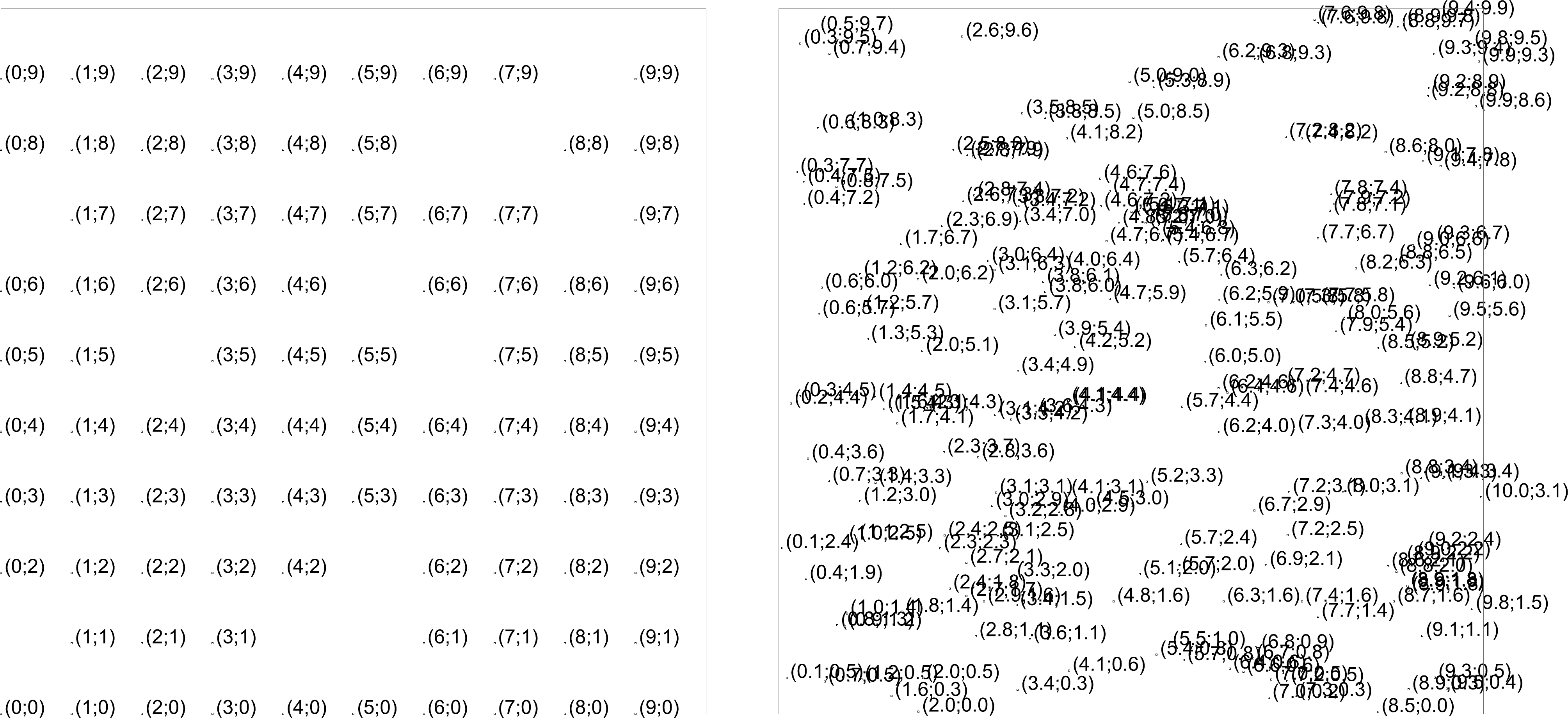
FIGURE 2 | Randomly generated coordinates.
On the left both w and l were given as exact numbers whereas on the right they were given as inexact numbers.

Another similar example but this with geometry we can actually see in our CAD would be a sphere made up of cuboids that have the bottom centre positioned at a point p but the top centre is randomly calculated. This cuboid-sphere is yet again a recursive function and will take as parameters the sphere’s centre p, the radius r and the number n of cuboids to be generated. We obviously need to specify the top centre point of the cuboids in spherical coordinates and have then range between 0 and 2pi.

(define (cuboid-sphere p r n)
  (if (= n 0)
      #t
      (cons
       (right-cuboid p 1 1 (+sph p
                                 r
                                 (random-range 0 2pi)
                                 (random-range 0 2pi)))
       (cuboid-sphere p r (- n 1)))))

This time, because 2pi is by nature an inexact number, we needn’t worry about using inexact numbers for our parameters. An example is shown in Figure 3:

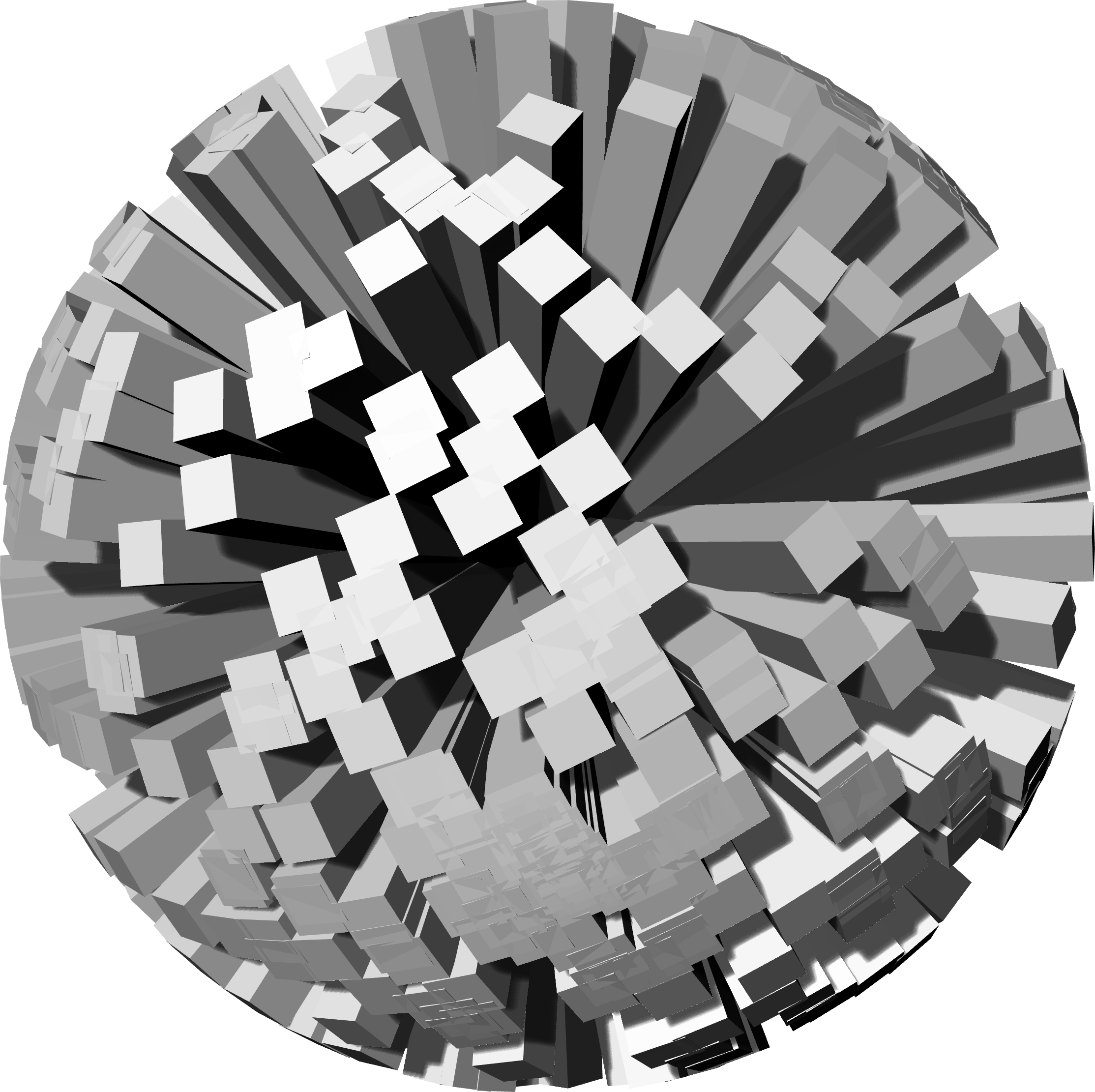
FIGURE 3 | A sphere made up of cuboids with one base positioned along the sphere’s surface.

One other usefulness in using random numbers in our design functions is to make choices. In several cases, although we have a general idea of what we want to do, we don’t concretely or necessarily now every detail. For example, if we wish create a function to generate a street flanked on both sides by buildings we don’t necessarily want to specify the type of building to be placed down during the execution of our function. One solution would be to have a family of buildings and then use a generator of random numbers to make the choice of which building to place down for us, in the vein of “If the random number is 0 then place building-1. If the random number is 1 then place building-2. Otherwise place building-3”.

As another example, imagine a Magic Eight-Ball^* and let’s try to write a function capable of simulating one. A standard Magic Eight-Ball has around 20 possible answers but we’ll reduce the number to 10. To create our generator of random answer we can use Rosetta’s function random-range and give it as limits 0 and 10 (not 9 since the top limit is out of the range). By using the cond form we can establish a decision based on the number generated. We can add an optional parameter for the question we want to ask. In Racket, to make a of a function parameter optional we place it inside a pair of straight brackets:

(define (magic-eight-ball question)
  (let ((n (random-range 0 10)))
    (cond ((= n 0) "It is certain.")
          ((= n 1) "Without a doubt.")
          ((= n 2) "Yes.")
          ((= n 3) "Ask again later.")
          ((= n 4) "Better not tell you now.")
          ((= n 5) "Don't count on it.")
          ((= n 6) "My reply is no.")
          ((= n 7) "Outlook not so good.")
          ((= n 8) "Very doubtfully.")
          ((= n 9) "No."))))

Now, we just need to invoke the function and write a yes-or-no question:

> (magic-eight-ball "Will I win the lottery")
"My reply is no."
> (magic-eight-ball "Will I ever find the meaning of life?")
"Ask again later."
> (magic-eight-ball "Am I a good person?")
"It is certain."
> (magic-eight-ball "Will the cafeteria be serving steak for lunch?")
"Yes."
> (magic-eight-ball "Can you really predict the future?")
"Very doubtfully."

With this example we can see how a generator of random number can be used to make decisions for us, although we probably shouldn’t rely much on them to predict our future. The range we define for the generator is actually very important since it affects the probability of each choice. In the last example each choice has the same probability of happening as the others (0.1%) because the random-range function is generating a set of numbers that’s the same as the number of choices. If we wanted to “rig” the option decision all we’d have to do is change the range. The function that tests the flipping of a coin is a good example to test this.

(define (flip-coin)
  (if (= (random-range 0 2) 0)
      "Heads"
      "Tails"))

(define (flip-fixed-coin)
  (if (= (random-range 0 6) 0)
      "Heads"
      "Tails"))

The flip-coin function is fair since both options “Heads” and “Tails” have a 50-50 chance of happening. The same does not apply to the flip-fixed-coin where the option “Tails” has an 80% chance of happening.

> (flip-coin)
"Tails"
> (flip-coin)
"Heads"
> (flip-coin)
"Heads"
> (flip-coin)
"Heads"
> (flip-coin)
"Tails"
> (flip-coin)
"Tails"
> (flip-coin)
"Heads"
> (flip-coin)
"Heads"
> (flip-coin)
"Heads"
> (flip-coin)
"Tails"
> (flip-fixed-coin)
"Heads"
> (flip-fixed-coin)
"Tails"
> (flip-fixed-coin)
"Tails"
> (flip-fixed-coin)
"Heads"
> (flip-fixed-coin)
"Tails"
> (flip-fixed-coin)
"Tails"
> (flip-fixed-coin)
"Tails"
> (flip-fixed-coin)
"Tails"
> (flip-fixed-coin)
"Tails"
> (flip-fixed-coin)
"Tails"
> (flip-fixed-coin)
"Tails"
> (flip-fixed-coin)
"Tails"
> (flip-fixed-coin)
"Tails"
> (flip-fixed-coin)
"Tails"
> (flip-fixed-coin)
"Tails"
> (flip-fixed-coin)
"Tails"
> (flip-fixed-coin)
"Tails"
> (flip-fixed-coin)
"Tails"
> (flip-fixed-coin)
"Tails"
> (flip-fixed-coin)
"Heads"

Let’s look at one final example, this time yielding a more graphical outcome. Truchet^* tiles are square tiles with a certain pattern that are placed next to each other to create a grid, much like decorative tiles used in architecture for covering wall or floors. These Truchet tiles are not rotationally symmetric, meaning that if you rotate one of them the direction of the pattern changes.

A common pattern used in these tiles is two circular arcs inscribed inside a square. Each arc is placed at opposing corners and has a radius that’s half the edge of the square. A tile can them be rotated to change its direction, as shown in Figure 2.

FIGURE 4 | A Truchet tile and its rotated equivalent

To create a composition with an interesting pattern we need to place tiles in a grid formation, alternating between both types of tile. Since the choice of tile is not something we want to specify ourselves we can have a generator of random numbers do it for us.

First let’s define two functions, each to model a type of tile seen in Figure 2. We will use the arc function to draw the arcs. The arcs on the left tile have domains [0 -pi/2] and [pi/2 pi/2]. Our tile1 function will have as parameters the tile insertion point p and edge l. We are not drawing the square of each tile since that would interfere with the reading of the final composition but feel free to do so:

(define (tile1 p l)
  (arc (+y p l) (/ l 2) 0 (- pi/2))
  (arc (+x p l) (/ l 2) pi/2 pi/2))

The tile2 function will be very similar but the arc domains change to [0 pi/2] and [pi pi/2]:

(define (tile2 p l)
  (arc p (/ l 2) 0 pi/2)
  (arc (+xy p l l) (/ l 2) pi pi/2))

Now we define a function tile-choice that will use a random function to make the choice of tile. Because we will want to explore different patterns in our final composition the top limit of the random generator will be a parameter – a. This way we will be able to control the probability of one tile being chosen over the other.

(define (tile-choice p l a)
  (if (= (random a) 0)
      (tile1 p l)
      (tile2 p l)))

The process of creating the grid of tiles is recursive and we have seen how to model it, in the tutorial A Brief Guide to Recursion . We will define two functions, one for generating one row of tiles and another to generate series of rows along the vertical axis. With these two functions we will be able to specify the number of tiles along the x axis – x-tiles, and along the y axis – y-tiles:

(define (row-tiles p l a x-tiles)
  (if (= x-tiles 0)
      #t
      (begin
        (tile-choice p l a)
        (row-tiles (+x p l) l a (- x-tiles 1)))))

(define (truchet-tiles p l a x-tiles y-tiles)
  (if (= y-tiles 0)
      #t
      (begin
        (row-tiles p l a x-tiles)
        (truchet-tiles (+y p l) l a x-tiles (- y-tiles 1)))))

Finally let’s define the function truchet-sample that besides creating a grid of tiles will also draw a square containing it and a legend showing what number was used for the parameter a. The square needs to have edges measuring (* l x-tiles) and (* l y-tiles) and be positioned at p. For creating the legend we can use the text function coupled with a format function for inserting the number given to a inside the text. We’ll also need to specify the text height and position.

(define (truchet-sample p l a x-tiles y-tiles)
  (rectangle p (+xy p (* x-tiles l) (* y-tiles l)))
  (text (format "a= ~A" a) (+y p (- (- l 5.5))) 2.8)
  (truchet-tiles p l a x-tiles y-tiles))

Now all we need to do is evaluate the following expressions to see the results shown in Figure 3:

(truchet-sample (xy 0 0) 10 1 10 10)
(truchet-sample (xy 115 0) 10 2 10 10)
(truchet-sample (xy 230 0) 10 3 10 10)
(truchet-sample (xy 0 115) 10 4 10 10)
(truchet-sample (xy 115 115) 10 5 10 10)
(truchet-sample (xy 230 115) 10 6 10 10)

FIGURE 5 | Several Truchet compositions by changing the a parameter.

Using the same reasoning we could also model a pseudo road network by creating a series of tiles for the roads and then placed them in a grid. If we consider three tiles – two with curves and one for an intersection, modelled using surfaces, as shown in the following figure:

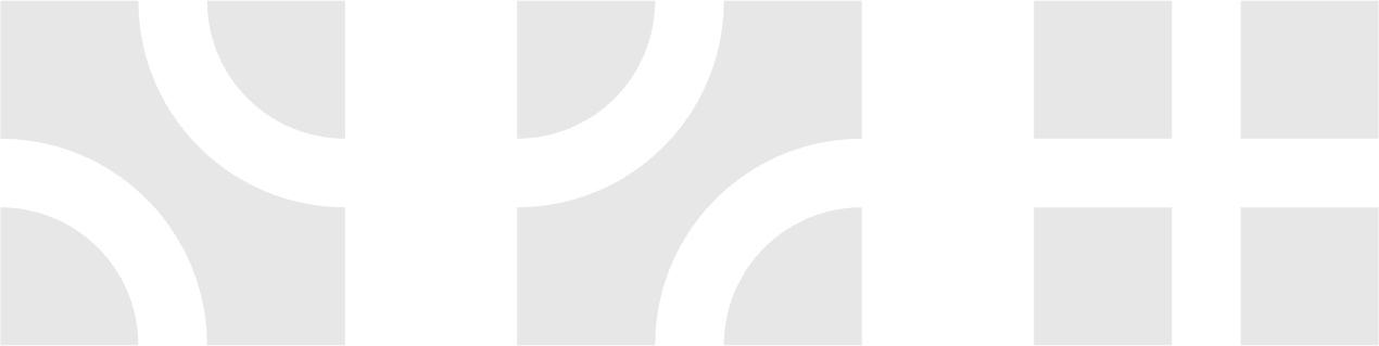
FIGURE 6 | Road tiles

We could use the exact same functions tile-choice, row-tiles and truchet-tiles for making the choice of tile and creating the grid. We will change the names however to road-choice, road-row and road-tiles as to avoid confusion. This time we have to make a choice between three tiles so in the function road-choice it is better to use a cond function instead of if . The functions needed to model our roads are as follows:

(define (road1 p l d)
  (let* ((l2 (- (/ l 2) (/ d 2)))
         (r (+ l2 d)))
    (surface-arc p l2 0 pi/2)
    (surface-arc (+xy p l l) l2 pi pi/2)
    (surface (line (+xy p l2 l) (+y p l) (+y p r))
             (line (+xy p l l2) (+x p l) (+x p r))
             (arc p r 0 pi/2)
             (arc (+xy p l l) r pi pi/2))))

(define (road2 p l d)
  (let* ((l2 (- (/ l 2) (/ d 2)))
         (r (+ l2 d)))
    (surface-arc (+y p l) l2 0 -pi/2)
    (surface-arc (+x p l) l2 pi/2 pi/2)
    (surface (line (+y p l2) p (+x p l2))
             (line (+xy p r l) (+xy p l l) (+xy p l r))
             (arc (+y p l) r 0 -pi/2)
             (arc (+x p l) r pi/2 pi/2))))

(define (road3 p l d)
  (let ((l2 (- (/ l 2) (/ d 2))))
    (union (surface-rectangle p l2 l2)
           (surface-rectangle (+xy p l l) (- l2) (- l2))
           (surface-rectangle (+y p l) l2 (- l2))
           (surface-rectangle (+x p l) (- l2) l2))))

And for making the choice and creating the grid:

(define (road-choice p l d a)
  (cond ((= (random a) 0)
         (road1 p l d))
        ((= (random a) 1)
         (road2 p l d))
         (else (road3 p l d))))

(define (row-roads p l d a x-tiles)
  (if (= x-tiles 0)
      #t
      (begin
        (road-choice p l d a)
        (row-roads (+x p l) l d a (- x-tiles 1)))))

(define (road-tiles p l d a x-tiles y-tiles)
  (if (= y-tiles 0)
      #t
      (begin
        (row-roads p l d a x-tiles)
        (road-tiles (+y p l) l d a x-tiles (- y-tiles 1)))))

If we generate a 10x10 grid using the road-tiles, with a choice parameter of a=5 we would get something like what can be seen in Figure 7:

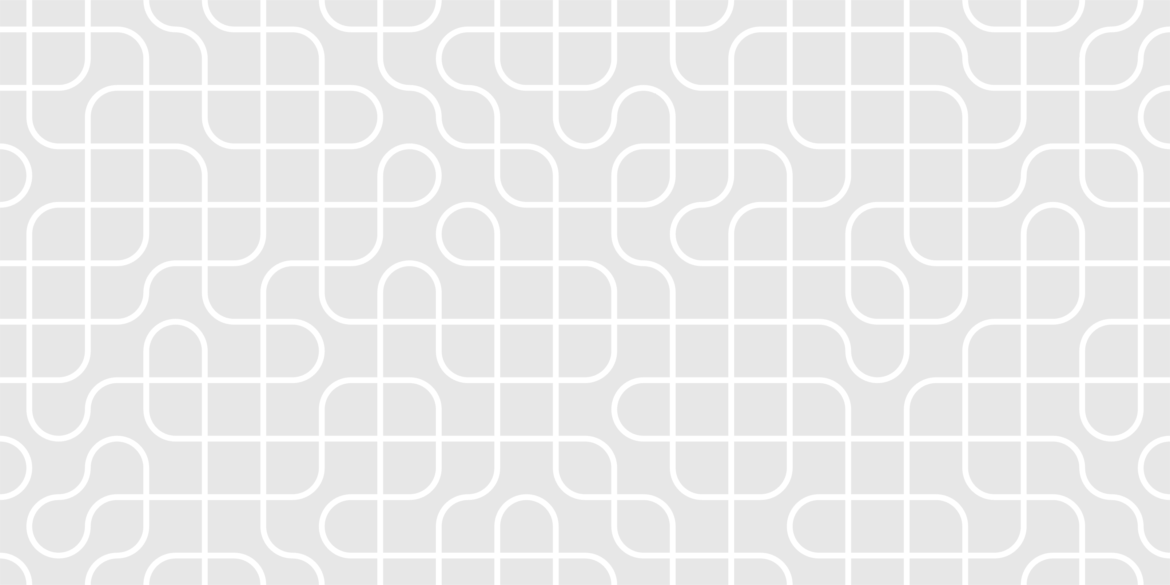
FIGURE 7 | A random road network

In the first section of this tutorial we said that the random function , or random-range for that matter, produces an apparently random number that’s based on the previously generated number. Both of these functions are examples of functions with history memory. They are required to know what the last generated value was in order to influence and generate the next one and that one will influence the one afterwards.

Whenever we use the form define we are creating an association between a name and a procedure. That procedure will then generate a result and we can trust that every time we invoke that name the same procedure will be executed every time. If we want our functions to have memory we need to have a way of changing that association so that the function will produce a result that is based on what the last execution produced. For that Racket provides the function set! which given an already assigned name and a new value will change the previous association to this new one. This is better understood with an example.

The Sierpinski Carpet is a famous bi-dimensional fractal discovered by Polish Mathematician Wacław Sierpiński which consists in constantly subdividing a square in 9 and removing the central square. The process is then repeated to each of the squares that resulted from the sub-division, as shown in Figure 8:

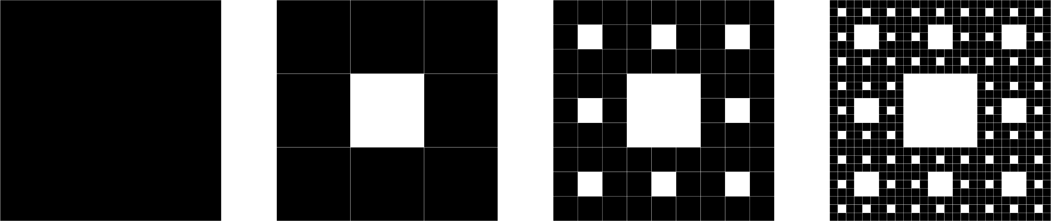
FIGURE 8 | Four Iterations of the Sierpinski Carpet

We will use this example to show how state can play an important part in our function. To model the Sierpinski Carpet we will employ surfaces to create a contrast between filled and unfilled regions. We can then us a series of subtraction operations for removing the smaller squares. The function will have as parameters the insertion point p (bottom left corner), the side length l and the number of subdivisions n. In the first iteration, when n=0, we need only use the surface-rectangle function to create a square of side l. In the next iteration we need to place a smaller square in the middle, with a side measuring 1/3 of l, and subtract it to the bigger square. We then perform 8 recursions, one for each square surrounding the middle one.

We start by defining a name called carpet1 that we will associate with procedure (surface-rectangle p (+xy p l l)). This is the first state of the recursion and after that we begin by defining the recursion. The stopping condition, because we are performing subtractions, will have to be the universal-shape since it is the neutral element for subtraction operations.

(define (sierpinski-carpet p l n)
  (define carpet1 (surface-rectangle p (+xy p l l)))
  (if (= n 0)
      (universal-shape)
      (begin
        ...)))

If n is not 0 then we proceed with the recursion. The first step is to place a smaller square at the middle of the large one, with sides measuring 1/3 of l and subtract it to the larger square. Then we need to change the association we made in (define carpet1 (surface-rectangle p (+xy p l l))) to the result of this subtraction, so that the next subtraction are applied to it and not to the original large square. This is where state needs to be introduced in our function. By using the operator set! we can change the meaning of carpet1 to the subtraction of the middle square to the larger square.

(define (sierpinski-carpet p l n)
  (define carpet1 (surface-rectangle p (+xy p l l)))
  (if (= n 0)
      (universal-shape)
      (begin
        (set! carpet1
              (subtraction carpet1
                           (surface-rectangle (+xy p (* l 1/3) (* l 1/3))
                                              (+xy p (* l 2/3) (* l 2/3)))))
        ...)))

Then we use the sierpinski-carpet 8 times, one for each of the 8 sub-squares surrounding the middle one. On the first time we use a subtraction operation again between carpet1 and sierpinski with p remaining at the same position, l now being (* l 1/3) and n being (- n 1). For the remaining recursions the position of p needs to change accordingly and we needn’t apply the subtraction again because, since it is part of the function sierpinski-carpet, the subtraction will be automatically and recursively applied to all the other regions of the square.

(define (sierpinski-carpet p l n)
  (define carpet1 (surface-rectangle p (+xy p l l)))
  (if (= n 0)
      (universal-shape)
      (begin
        (set! carpet1
              (subtraction carpet1
                           (surface-rectangle (+xy p (* l 1/3) (* l 1/3))
                                              (+xy p (* l 2/3) (* l 2/3)))))
        (subtraction carpet1 (sierpinski-carpet p (* l 1/3) (- n 1)))
        (sierpinski-carpet (+y p (* l 1/3)) (* l 1/3) (- n 1))
        (sierpinski-carpet (+y p (* l 2/3)) (* l 1/3) (- n 1))
        (sierpinski-carpet (+xy p (* l 1/3) (* l 2/3)) (* l 1/3) (- n 1))
        (sierpinski-carpet (+xy p (* l 2/3) (* l 2/3)) (* l 1/3) (- n 1))
        (sierpinski-carpet (+xy p (* l 2/3) (* l 1/3)) (* l 1/3) (- n 1))
        (sierpinski-carpet (+x p (* l 2/3)) (* l 1/3) (- n 1))
        (sierpinski-carpet (+x p (* l 1/3)) (* l 1/3) (- n 1)))))

We can now test this function and try to reproduce Figure 8. Just be careful with the number of subdivisions since the computation needed increases exponentially as the parameter n increases.

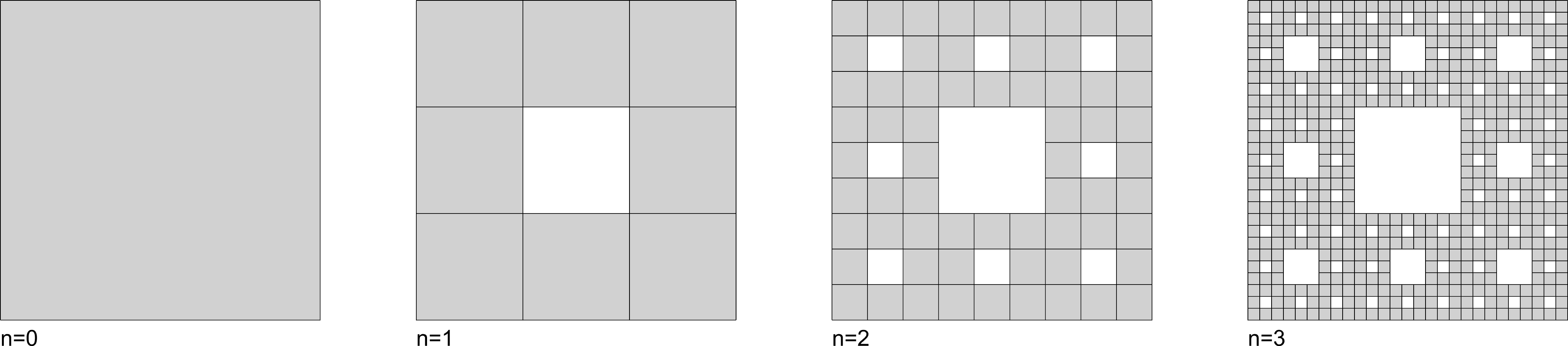
FIGURE 9 | The Sierpinski Carpet modelled with surfaces

In this tutorial we saw how we can incorporate randomness into our programs, whether it is for randomly assigning values to parameters, randomly generating data or for making choices. We have also learned the concept of state and how to introduce such behaviour in our function by using the operator set! .

In the next tutorial we will be looking at the fundamentally important subject that is data structures. Stay tuned!