ROSETTA

Contents:
• Part I - Translation
• Part II - Scale
• Part III - Rotation
• Part IV - Mirror
• Part V - Slice

Forms that we create using Rosetta don’t have to be definite in their character, i.e., It is possible to modify any geometry we create in terms of its position, scale and orientation, even after we’ve created them. Rosetta provides the functions move , scale , rotation and mirror for performing translations, scaling, rotations and reflections, respectively. These operations act upon the provided geometry thus modifying it; they don’t produce new shapes. If we want to perform any of these operations but still maintain the original geometry then we would have to first create a copy of that geometry, using the function copy-shape , and then apply the transformation to that copy. The copied geometry will be placed at exactly the same location as the original one so in the CAD application you’d see two coincidental objects.

The move function moves geometry from one point to another by applying a translation vector to all points of that object. If we consider a sphere that we wish to move from its original position to another then we can write:

(move
 (sphere (xyz 1 3 0) 2)
 (xyz 5 5 5))

Or alternatively:

(move
 (copy-shape (sphere (xyz 1 3 0) 2))
 (xyz 5 5 5))

Obviously, seeing as we can already control the position of the sphere when specifying its insertion point, it would be much easier to just write:

(sphere (xyz 5 5 5) 2)

Or we could also use the function +xyz using the sphere’s insertion point as reference:

So we can see that there are many ways at moving geometry around in space, either at the point of its creating or afterwards. It is therefore important to understand which situation calls for a certain translation procedure. In the previous example of a sphere it is clear that using the move function is not the most efficient way but in more complex cases it may be easier to consider that our geometry is initially created at specific location, the origin for example, and then moved to another location.

Let’s consider that we want to model a triple cross made up of cylinders and we want to be able to specify its position and radius. We could simply write:

(define (triple-cross p r)
  (cylinder p
            r
            (+z p (* 10 r)))
  (cylinder (+x p (- (* 5 r)))
            r
            (+x p (* 5 r)))
  (cylinder (+xz p (- (* 3 r)) (* 5 r))
            r
            (+xz p (* 3 r) (* 5 r)))
  (cylinder (+xz p (- (* 1.5 r)) (* 10 r))
            r
            (+xz p (* 1.5 r) (* 10 r))))

(triple-cross (xyz 5 5 5) 2)

And now we can place it wherever we want simply by changing the p parameter. An alternative way of defining this function without the insertion point p would be to consider the cross positioned at the origin, and for that we use the u0 ^* function, and apply a translation with move to a list containing the cylinders:

(define (triple-cross r)
  (move
   (list (cylinder (u0)
                   r
                   (z (* 10 r)))
         (cylinder (x (- (* 5 r)))
                   r
                   (x (* 5 r)))
         (cylinder (xz (- (* 3 r)) (* 5 r))
                   r
                   (xz (* 3 r) (* 5 r)))
         (cylinder (xz (- (* 1.5 r)) (* 10 r))
                   r
                   (xz (* 1.5 r) (* 10 r))))
   (xyz 5 5 5)))

(triple-cross 2)

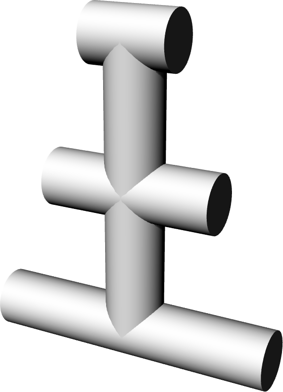
FIGURE 1 | A triple cross

The operation of scaling with scale uniformly increases or decreases the dimension of an entity when provided with a scaling factor – higher than 1 for increasing and lower to decrease the size. It is important to note that performing a scaling modification to an object might change its position in space as well. To avoid this small side effect we can first apply a translation to move the object to the origin and then, after performing the scale operation, place the object back into its original position. Taking the triple-cross example once more we can simplify its definition by using the scale operation. The cross is already placed at the origin leaving the radius r as the only parameter. If we use a unitary radius instead then we can control the radius with a scale operation:

(define (triple-cross)
  (list (cylinder (u0) 1 (z 10))
        (cylinder (x -5) 1 (x 5))
        (cylinder (xz -3 5) 1 (xz 3 5))
        (cylinder (xz -1.5 10) 1 (xz 1.5 10))))

(scale (triple-cross) 2)

Note that we had to place all the geometry of the cross inside a list, otherwise the scale would only have been applied to the last created cylinder instead of all four. Instead of a list we could also have performed a union operation which is something we’ll see how to do in the next tutorial.

The rotation is another very useful function which rotates every point in an object in a circular motion, by providing the rotation angle and two points that define the rotation axis. By omission the rotation angle is along the Z axis.

If we wanted to stack cubes on top of each other, each with a slightly different rotation, we could write:

(right-cuboid)
(move (rotate (right-cuboid) pi/6 (u0) (uz)) (z 1))
(move (rotate (right-cuboid) (* 2 pi/6) (u0) (uz)) (z 2))
(move (rotate (right-cuboid) (* 3 pi/6) (u0) (uz)) (z 3))
(move (rotate (right-cuboid) (* 4 pi/6) (u0) (uz)) (z 4))

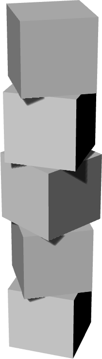
FIGURE 2 | Stacked and rotated cubes

Each cuboid is first created at the origin and then move to its rightful location with the help of the move tool.

We also have the mirror function which creates a reflection of an object by specifying a point and a vector normal to the plane of reflection. If omitted, the mirror will be performed along the XY plane. We can use the mirror function to create the following 2D shape, where we just draw one quarter of it and then use several mirrors to create the remaining three quarters:

(mirror
 (mirror
  (mirror
   (list
    (surface-polygon (xy 3 0)
                     (xy 15 0) 
                     (xy 10 5)
                     (xy 6 1)
                     (xy 1 6)
                     (xy 5 10)
                     (xy 0 15)
                     (xy 0 3))
    (regular-prism 4 (xyz 6 6 -1) 2 0 2)
    (regular-prism 4 (xyz 0 0 -0.5) 1 0 1))
   (u0) (x 1))
  (u0) (y 1))
 (u0) (x -1))

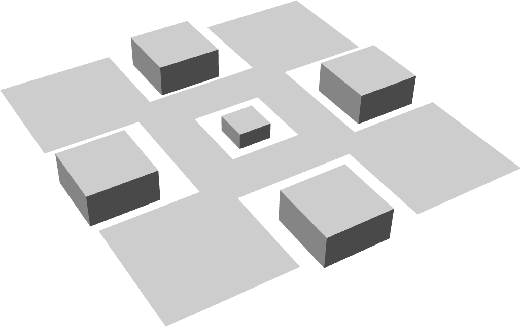
FIGURE 3| A mirrored shape

As another example let’s suppose we want to model a star shaped pyramid, composed of three stacked irregular pyramid frustums. For this we will decompose the problem into three parts: the first part is to model one quarter of a step, the second part is to stack three steps on top of each other and the last part is to perform a reflection to model the remaining quarters of our pyramid.

To model one step we use the cuboid function since the footprint is irregular and couldn’t be modelled using the regular-pyramid-frustum . The step function will take as parameters the insertion point p, the base side length b, the top side length t and the step height h.

(define (step p b t h)
  (let ((b2 (* 1.2 b))
        (t2 (* 1.2 t)))
    (cuboid p (+y p (- b)) (+xy p b2 (- b2)) (+x p b)
            (+z p h) (+yz p (- t) h) (+xyz p t2 (- t2) h) (+xz p t h))))

For stacking two more steps on top of the first one we can use the move and scale functions. After creating one step we place another scaled down step on top of it and another one even smaller on top of that one.

(define (steps p b t h)
  (list (step p b t h)
        (move
         (scale (step p b t h) 0.7 (+z p h))
         (+xyz p (/ h 3) (- (/ h 3)) (* 0.7 h)))
        (move
         (scale (step p b t h) 0.5 (+z p h))
         (+xyz p (/ h 3) (- (/ h 3)) (* 1.2 h)))))

Once again, we placed the geometry inside a list so that in the next part we can perform a reflection to all the steps and not just the last one. To create the remaining quarters of our pyramid we need only use the function mirror :

(define (star-pyramid p b t h)
  (mirror
   (mirror
    (mirror (steps p b t h) (u0) (y -1))
    (u0) (x 1))
   (u0) (y 1)))

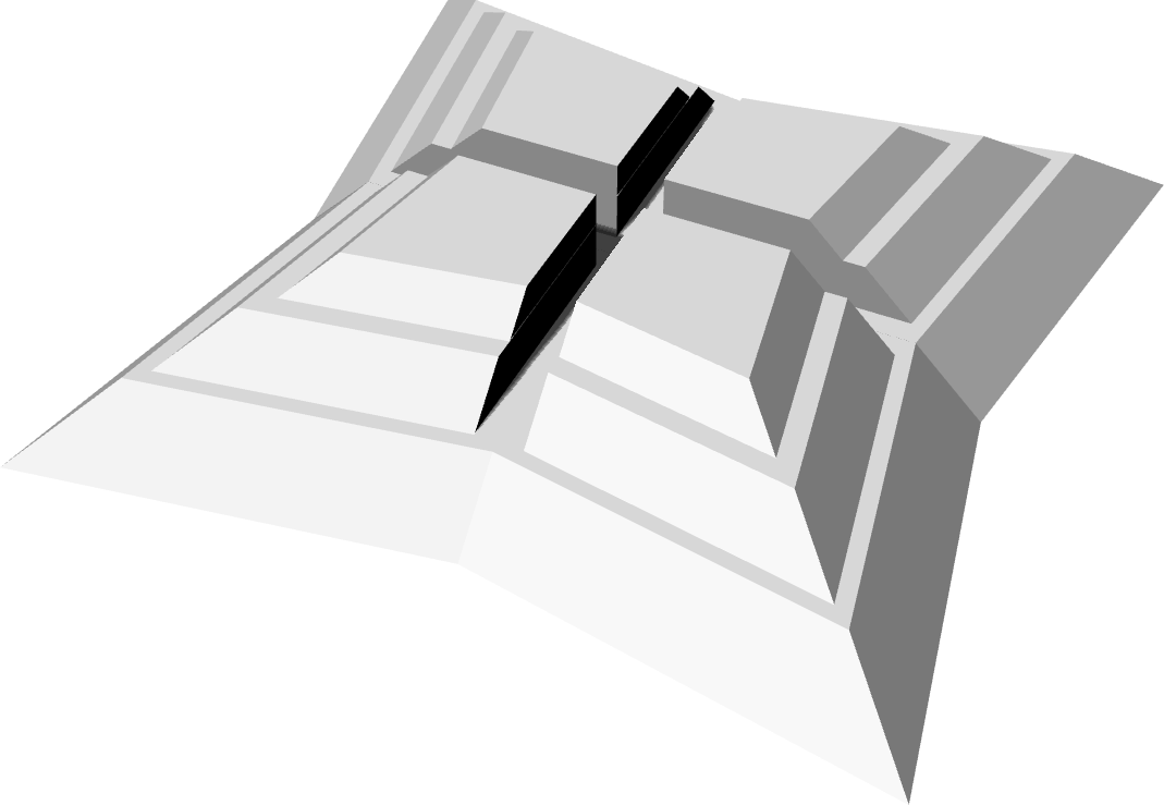
FIGURE 4| A star-shaped pyramid

One of the advantages of using 3D transformations over other alternative methods is the cut back in our effort to model a certain shape. In the last example we could just as well have drawn the entire figure using other modeling methods but understanding that this figure has certain degrees of symmetry means we don’t have to model the entire shape in one sitting. Instead, it’s much more practical to model only part of it and then use 3D transformation operations to generate the rest. This also means that any future changes we wish to make in our models need only be applied to the part that is then being transformed.

In the next tutorial we will be introducing the concept of Constructive Geometry and the functions that allow the computation of Boolean operations such as unions, intersections and subtractions. When ready please click the link below.