ROSETTA

Contents:
• Part I - Underlying urban grid
• Part II - Controlling height with a complementary surface
• Part III - Modelling the terrain

In part I we looked at a method of generating random cities using recursion. It generates a fairly realistic result especially if we have the height of building varying according to a distribution function. However, we are pretty much stuck to the same model of flat urban grid that may not reflect what we wish to do. Say we wish to generate a city that’s not set on a flatsurface but rather on a waved surface that simulates natural topographic features of a site. Using the method we implemented in part I does not allow this. In this part however we will explore an alternative method that doesn’t rely on recursion to generate a grid of buildings but rather using surface processing algorithms. This method is much more flexible and allows for much more variation since we will use high-order functions to choose the type of surface onto which we wish to generate the city.

Launch DrRacket, load Rosetta and choose you CAD. It might be a good idea to also add (erase-2d-top) to quicken the geometry generation process in you CAD.

#lang racket

(require (planet aml/rosetta))
(backend rhino5)
(erase-2d-top)

So, at the end of the previous tutorial we finished with five fundamental functions: building0 that generates a box-shaped building, building1 that generates a cylindrical building, building which makes a random choice of which building to place down, buildings-row that recursively generates one row of buildings and finally city-grid that creates the entire grid of buildings. We do not need to chuck all these functions away for this tutorial. In fact the only ones we will not need are the last two since they rely on recursion and we don’t want that anymore for this project. So, if you are using the same Racket file you created last time, please go ahead and either delete those functions or document them. To the others we will just have to make a few minor changes.

The fundamental thinking process for this tutorial is similar to previous tutorials that work with surface processing and mapping techniques: we’ll have a parametric equation of a surface generating a matrix of points in space (this will simulate our site terrain), we will have the function iterate-quads creating 4-tuples of points from that matrix (thus defining a cell that will be used as a city block), and finally, taking those 4 points we will define a building to be placed. In Figure 1 we have a quick sketch of this paradigm:

FIGURE 1 | Sketch of a city processed along a surface

Since we’ll be working with quads of points that, in most cases, will not define a planar shape, it might be a good idea to modify our previous building0-blocks and building1-blocks functions so that instead of having their insertion point p be one of the corners of a city block, actually use the quad’s middle point as the insertion point. Let’s quickly define a function that, given the four points that define one quad, computes its centre point. In Figure 2 we can see how this is calculated: the centre point of a 4 side polygon will be the middle point of the middle point of its two diagonals.

FIGURE 2 | How to calculate the centre point of a 4 side polygon

(define (quad-centre p0 p1 p2 p3)
  (pts-average
   (pts-average p0 p2)
   (pts-average p1 p3)))

And the function for calculating the average point between two points:

(define (pts-average p0 p1)
  (/c (+c p0 p1) 2))

Now what’s left is to do is modify our building0-blocks and building1-blocks functions to have the buildings base centre point as its insertion point. We could still use the box function but it is much more convenient if we use the right-cuboid function instead:

(define (building0-blocks p l w h n-blocks)
  (let* ((top-h (* (random-range 0.2 0.8) h))
        (top-l (* (random-range 0.7 1.0) l))
        (top-w (* (random-range 0.7 1.0) w))
        (top-p (+z p top-h)))
    (if (= n-blocks 1)
        (right-cuboid p l w h)
        (begin
          (right-cuboid p l w top-h)
          (building0-blocks top-p top-l top-w top-h (- n-blocks 1))))))

(define (building1-blocks p l h n-blocks)
  (let* ((top-h (* (random-range 0.2 0.8) h))
        (top-l (* (random-range 0.7 1.0) l))
        (top-p (+z p top-h)))
    (if (= n-blocks 1)
        (cylinder p (/ l 2.0) h)
        (begin
          (cylinder p (/ l 2.0) top-h)
          (building1-blocks top-p top-l top-h (- n-blocks 1))))))

We obviously need the functions building0, building1 and building as well, but we needn’t make any changes to them:

(define (building0 p l h)
  (building0-blocks p l l h (random-range 1 6)))

(define (building1 p l h)
  (building1-blocks p l h (random-range 1 6)))

(define (building p l h)
  (if (= (random 5) 0)
      (building0 p l h)
      (building1 p l h)))

The next thing we need to think of is our terrain. The idea is to use a parametric surface that we can easily process to create the points we need. There are obviously many surfaces to choose from so let’s use a simple open-surface defined parametrically as:

Where a is a parameter to control the “intensity” of the curvature and (u,v) is the surface domain. The function can easily be implemented in Racket:

(define (terrain-surface p a u0 u1 n v0 v1 m)
  (map-division
   (lambda (u v)
     (+xyz p
           u
           v
           (* a (+ (sin (+ u v)) (exp (/ (abs (- u 1)) 10)) (sin (- v 1)))))) 
   u0 u1 n
   v0 v1 m))

Using Rosetta’s surface-grid function we can have a quick look at what shapes we can get create by changing the parameter a:

FIGURE 3 | How to calculate the centre point of a 4 side polygon

The second example, where a = 0.2 seems like a good choice since it isn’t too steep but still has a nice curvature. If you wish the terrain to be flat just have a be 0.

One extra function we need to define though is the function that will generate a building by receiving as inputs the 4 points that constitute the cell in which a building is placed. A few considerations regarding this: the size of each cell will be controlled by the previous function that generates the surface of points. Naturally, the number of times we choose to divide u and v domains the smaller each cell will be. Therefore, it might be advisable to have the building’s length and height parameters, l and h respectively, not as parameters specified by the user but rather as local variables that change according to the size of a cell. The building-quad function that we’ll now define must take this in consideration and use the smaller cell side length as a reference:

(define (building-quad p0 p1 p2 p3 h)
  (let ((c (quad-centre p0 p1 p2 p3))
        (l (* (min (distance p0 p1) (distance p0 p3)) 0.8)))
    (building c l h)))

The parameter l is defined as being the minimum cell side multiplied by a factor the here we decided to be 0.8. The parameter h is defined as being triple the value of l. Obviously you are free to change these values to ones you see more fit. The building insertion point is c, the centre point of the cell.

Next we need the iterate-quads function that will take for parameters the building-quad function and apply it to the points generated by the terrain-surface function. In case you don’t have the iterate-quads function handy here it is:

(define (iterate-quads f ptss)
  (for/list ((pts0 ptss)
             (pts1 (cdr ptss)))
    (for/list ((p0 pts0)
               (p1 pts1)
               (p2 (cdr pts1))
               (p3 (cdr pts0)))
      (f p0 p1 p2 p3))))

Finally, our new city-grid function will be defined in terms of the two previous functions:

(define (city-grid srf h)
  (surface-grid srf)
  (iterate-quads
   (lambda (p0 p1 p2 p3)
     (let ((l (max (distance p0 p1) (distance p0 p3))))
       (building-quad p0 p1 p2 p3 h)))
   srf))

This function uses the iterate-quad to process the four corners of a building block – p0, p1, p2 and p3, and those points are used by the building-quad function to model a building in each cell provided by the srf parameter. Notice that we also included a surface-grid so that we can actually see our “terrain” modelled. In Figure 4 we can see the result.

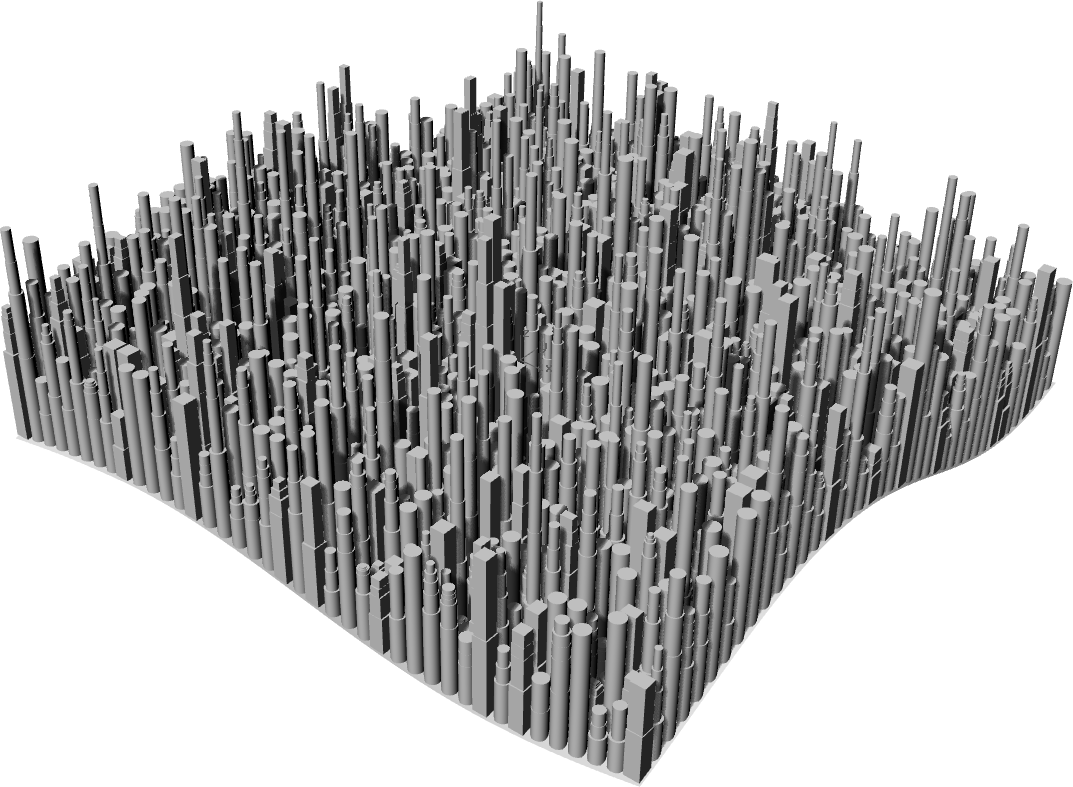
FIGURE 4 | A grid of buildings generated along a surface

The city we have so far is looking decent as it is but suppose we wish to add some height variation to our buildings. We could once again use a distribution function and insert it in the building function but since that in this tutorial we are experimenting with surface processing methods let’s try out a different method along those lines. If we look at the function building-quad we see that it creates a building inserted at a point c that is nothing less than a quad centre point of a series of points being generated and processed. The iterate-quads function takes those points, given by the function terrain-surface, and processes them in tuples of 4. With those four points a building can be created. Suppose now that above the terrain surface we have another surface being processed in quads, and the distance between the middle points of those quads and the quads on the terrain-surface is the height given to the building-quad function. That way, the height of the buildings will vary since the geometry of the new surface, which we will henceforth call height-surface, is what determines the overall height of each building. Figure 5 shows a diagram of this paradigm.

FIGURE 5 | Diagram of how to use a surface to determine the height of each building

The two surfaces are independent from one another but since a building will now need to have both 4 points on the bottom and top surfaces to determine its size and height then it might be convenient to have two pairs of 4-tuples being processed at the same time instead of just the four on the bottom surface. But the function we have at the moment, which iterates points, only does so for four points and not eight. Let’s change that:

(define (iterate-2-quads f ptss1 ptss2)
  (for/list ((pts0 ptss1)
             (pts1 (cdr ptss1))
             (pts2 ptss2)
             (pts3 (cdr ptss2)))
    (for/list ((p0 pts0)
               (p1 pts1)
               (p2 (cdr pts1))
               (p3 (cdr pts0))
               (p00 pts2)
               (p11 pts3)
               (p22 (cdr pts3))
               (p33 (cdr pts2)))
      (f p0 p1 p2 p3 p00 p11 p22 p33))))

This new iteration function will take two sets of points and process them in pairs of four points: p0, p1, p2 and p3 will be the four points on the terrain-surface and p00, p11, p22 and p33 will be the four points on the height-surface. A given function f, which will later be the building function, will then be applied to all eight points.

For the height-surface let’s consider another open parametric surface given by:

Where once again a controls the intensity of the curvature and (u,v) are the surface domains. Translated into Racket this formula will be:

(define (height-surface p a u0 u1 n v0 v1 m)
  (map-division
   (lambda (u v)
     (+xyz p
           u
           v
           (* (/ 4.0 10) (* a (sin (* u v))))))
   u0 u1 n
   v0 v1 m))

(Note that in both this function and the terrain-surface we could have placed fixed domains since in our case we want both surfaces to have the same domains and number of divisions. We haven’t done so to not restrict their use in other contexts. Just keep in mind when invoking the two functions you should give them the same domains and number of divisions.)

We now have everything we need to define the new city-grid function. There is however another thing to consider: the top surface, which will serve to calculate the height, can, and will probably have in most cases, a different geometry than the bottom surface. It is therefore foreseeable that the two might intersect each other if we don’t space them out enough. On these occasions where the points on the site-surface are higher than the points on the height-surface we need to think what we want to happen. In this case it probably makes more sense to have no building whatsoever. We can therefore create a conditional statement that says: “If the z-coordinate of the top centre point is smaller or equal to the z-coordinate of the bottom centre point then don’t do anything. Otherwise place a building with a height equal to the distance between the two centre points”. The city-grid will then have the following definition:

(define (city-grid srf-terrain srf-height)
  (surface-grid srf-terrain)
  (iterate-2-quads
   (lambda (p0 p1 p2 p3 p00 p11 p22 p33)
     (let ((c0 (quad-centre p0 p1 p2 p3))
           (c1 (quad-centre p00 p11 p22 p33)))
       (if (<= (cz c1) (cz c0))
           #t
           (building-quad p0 p1 p2 p3 (distance c0 c1)))))
   srf-terrain srf-height))

We need only to give this function the two surfaces and see the results:

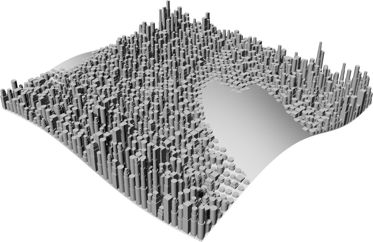
FIGURE 6 | City being generated between two surfaces

One aspect of this model that does not look very elegant is the fact that the terrain surface is open and we can see underneath it. If you were physically creating a mock-up model of this city, or rather of its terrain, you wouldn’t leave the sides of the terrain open so should consider this and try to implement it in our code. This is easy to do provided we have the edge curves of the surface that forms our terrain. We could then interpolate those edges with their projected equivalents on the xy-plane and that would model the four side skirts.

If we think that the parametric equation is generating a matrix of points which are subsequently used to model the terrain, it becomes easy to see that in order to create the edge curves, we need only access the first and last lines in that matrix. We could use the spline function to interpolate those points and that would give us the two terrain edges in the horizontal direction. To get the other two edges on the vertical direction we need only transpose the matrix of points and repeat the process of retrieving the first and last lines of points. So, to start, we need to define the function capable of transposing a matrix:

(define (transpose-matrix matrix)
  (if (null? (car matrix))
      (list)
      (cons (map car matrix)
            (transpose-matrix (map cdr matrix)))))

It is now easy, using Racket’s first and last functions, which retrieve the first element of a list respectively, to create a first draft of the function that will model the terrain. We can use the Rosetta’s function spline to interpolate those points and draw the edges:

(define (terrain-model srf)
  (spline (first srf))
  (spline (last srf))
  (spline (first (transpose-matrix srf)))
  (spline (last (transpose-matrix srf))))

We can see in Figure 6 what we have so far.

FIGURE 7 | Terrain surface edges

We’re on the right path to model the side skirts of the terrain but there is something else we need and those are the corresponding edges on the XY-plane. One thing we could do is use the same previous function but upon invoking it we would specify that a, the parameter that controls the terrain’s curvature, is equal to 0. This would give as a flat surface on the XY-plane from which we could, again, extract the first and last points and draw the edges. However, this is not the most appropriate way of doing it for the reason that the function as it is, and it is more convenient that it stays that way, only receives that one parameter srf. Obviously we could change that parameter srf and include as alternatives all the parameters that specify the terrain surface but that would result in a function with repetitive and excessive code:

(define (terrain-model p a u0 u1 n v0 v1 m)
  (spline (first (terrain-surface p a u0 u1 n v0 v1 m)))
  (spline (first (terrain-surface p 0 u0 u1 n v0 v1 m)))
  (spline (last (terrain-surface p a u0 u1 n v0 v1 m)))
  (spline (last (terrain-surface p 0 u0 u1 n v0 v1 m)))
  (spline (first (transpose-matrix (terrain-surface p a u0 u1 n v0 v1 m))))
  (spline (first (transpose-matrix (terrain-surface p 0 u0 u1 n v0 v1 m))))
  (spline (last (transpose-matrix (terrain-surface p a u0 u1 n v0 v1 m))))
  (spline (last (transpose-matrix (terrain-surface p 0 u0 u1 n v0 v1 m)))))

You can see how unappealing this function looks with all that repetitive code. Normally, when there is code being repeated over and over it’s a good sign that it can be simplified. Let’s go back to having just the srf as the single parameters and think how to do this differently. There is a very simple way of having the points we need in terms of the terrain surface, and that is to take all those generated points and project them onto the XY-plane where z=0. If we create a function capable of doing this then we just need to map it onto the matrix of points and retrieve the first and last lines from that new matrix. This flatten-point function is easy to define:

(define (flatten-point p)
  (if (<= (cz p) 0)
      (+z (+z p (- (cz p))) -0.7)
      (+z p (- (cz p)))))

Considering that there may be cases where the surface may be below the z=0 horizontal plane, we included a small conditional statement in the previous function to say that, if the surface is indeed below that plane, then first project the points onto the z=0 plane and add a value of 0.7 so the terrain model has some thickness. Now using the function map we can apply it to the first and last elements of the point matrix:

(define (terrain-model srf)
  (spline (first srf))
  (spline (map flatten-point (first srf)))
  (spline (last srf))
  (spline (map flatten-point (last srf)))
  (spline (first (transpose-matrix srf)))
  (spline (map flatten-point (first (transpose-matrix srf))))
  (spline (last (transpose-matrix srf)))
  (spline (map flatten-point (last (transpose-matrix srf)))))

This function is looks much neater than the other alternative although it still has some repeated code and functions. We will simplify it in a few moments so for now let’s stick with what we have. With all the edge curves we need we can now perform an interpolation using the function loft and model all four side skirts. We can also add the terrain surface using surface-grid :

(define (terrain-model srf)
  (surface-grid srf)
  (loft (list (spline (first srf))
              (spline (map flatten-point (first srf)))))
  (loft (list (spline (last srf))
              (spline (map flatten-point (last srf)))))
  (loft (list (spline (first (transpose-matrix srf)))
              (spline (map flatten-point (first (transpose-matrix srf))))))
  (loft (list (spline (last (transpose-matrix srf)))
              (spline (map flatten-point (last (transpose-matrix srf)))))))

To make this function simpler we could take out the sequence (loft (list (spline ...))) and put it in a separate function and we could also define a local variable for the transposed matrix of srf:

(define (model-skirt pts)
  (loft (list (spline pts)
              (spline (map flatten-point pts)))))

(define (terrain-model srf)
  (surface-grid srf1)
  (model-skirt (first srf))
  (model-skirt (last srf))
  (let ((srf2 (transpose-matrix srf)))
    (model-skirt (first srf2))
    (model-skirt (last srf2))))

We can now include this function in the city-grid:

(define (city-grid srf-terrain srf-height)
  (terrain-model srf-terrain)
  (iterate-2-quads
   (lambda (p0 p1 p2 p3 p00 p11 p22 p33)
     (let ((c0 (quad-centre p0 p1 p2 p3))
           (c1 (quad-centre p00 p11 p22 p33)))
       (if (<= (cz c1) (cz c0))
           #t
           (building-quad p0 p1 p2 p3 (distance c0 c1)))))
   srf-terrain srf-height)
  #t)

We have also included a Boolean #t at the end so that Racket doesn’t return the value of every geometry it created. In Figure 6 we can see the final result:

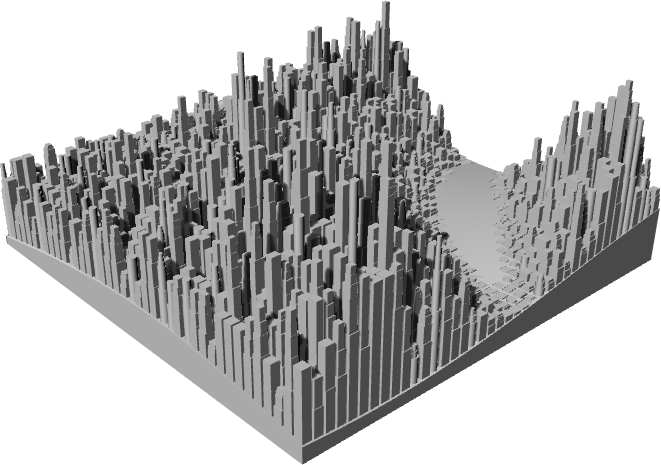
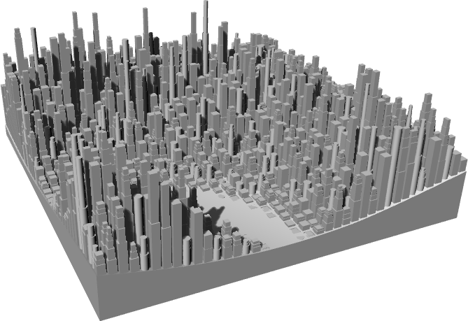
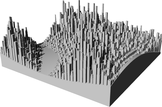
FIGURE 7 | Subtraction and intersection of spheres

Obviously we can now play around with the functions we created, namely the ones that create the terrain geometry and control the building height, in order to obtain different results. The following figures show some examples obtained by either specifying new terrain/height surfaces or simply by changing some parameters in the functions we already have.

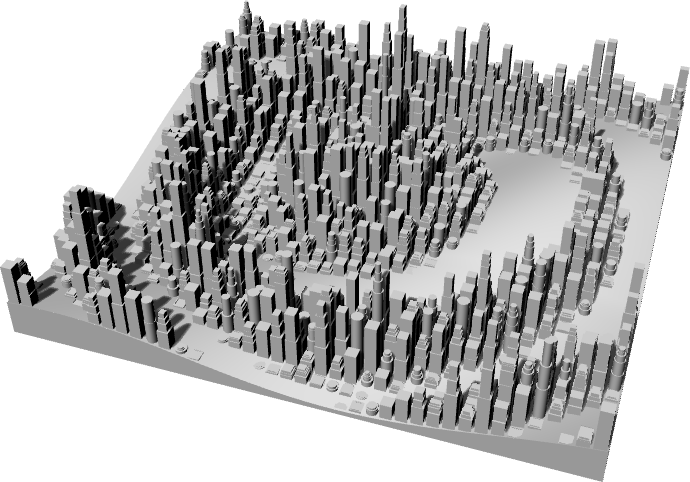
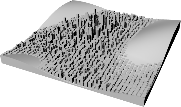
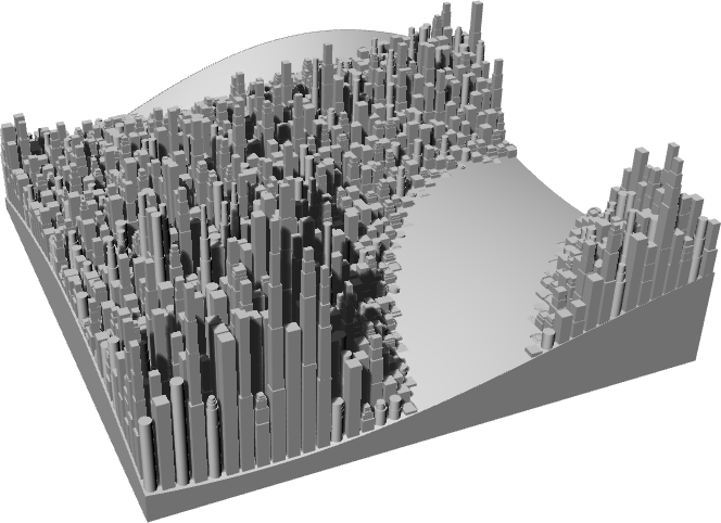
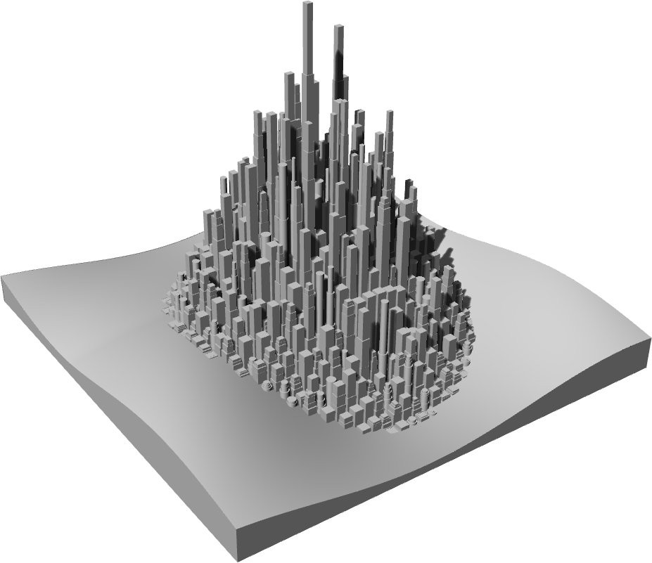
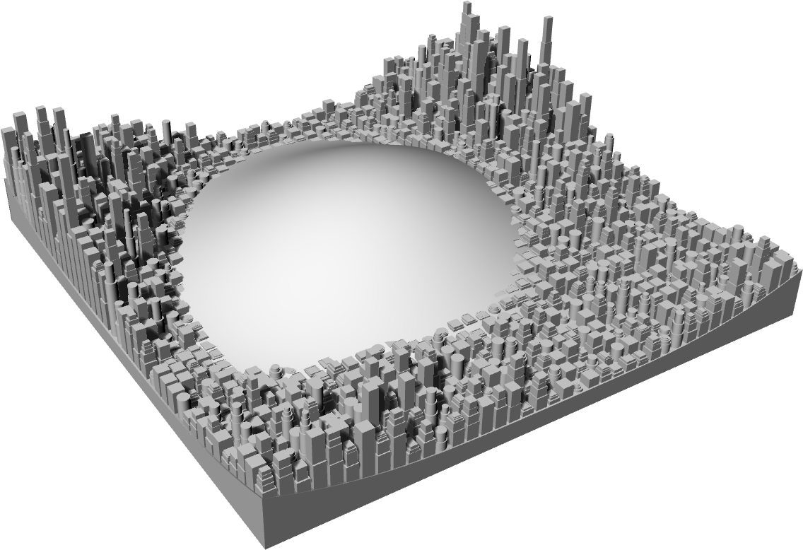
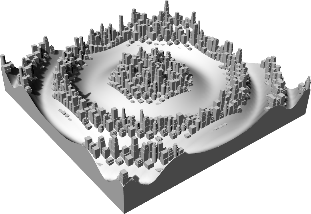
FIGURE 8 | Examples of cities with different parameters