ROSETTA

Contents:
• Part I – Setting up a render with Rosetta
• Part II – Rendering in Rhino
• Part III – Rendering in AutoCAD
• Part IV – Setting up an animation with Rosetta

If you are working on a project there’s a good change that, by the end of it, you want to produce nice appealing images to present your work in a publication or website. With Rosetta it is easy to set up your model so that you can automatically generate a rendered image of your models.

For this tutorial you will need to have a model to work with. If you don’t have a model of your own handy then you can download one below:

• PAVILLION RENDER TEST RHINO.RKT ⇦ (choose this file if you are using Rhino)
• PAVILLION RENDER TEST AUTOCAD.RKT ⇦ (choose this file if you are using AutoCAD)

In the Racket file you downloaded you should see a document divided into two parts. The “Utilities” part contains a number of utility functions needed for other’s to work. Some of these you should already be familiar with if you followed previous tutorials. The section part, named “Pavilion” contains the actual functions for generating the building we will be using for this tutorials. The functions in the “Roof” section generate the roof of the building and its structure in the form of a cylindrical sine wave. The functions inside the “Glazing” section create the outside facade of the building as a curtain wall, divided into a given number of windows. The section “Courtyard” contains all the functions for generating the central courtyard together with a decorative sculptural piece. Finally the “Final Building” gathers all those previous functions together and generates the entire building. The parameters are as follows:

The process of rendering an image using Rosetta can be made two ways: you can set up and render you project directly from DrRacket or, alternatively, you can just do the setting up in DrRacket and then manually render you project in the CAD software. The later gives you more freedom for preparing materials and adjusting rendering options but can be time consuming if you wish to render several images. The first method is much faster since the whole process can be automated and set to produce any number of renders you want effortlessly. What is important to keep in mind is that the final result will be different depending on what software you are using. A render in AutoCAD will produce different result than a render generated in Rhino for example, and the process to set up the appropriate materials and ender setting will also be different.

The workflow for producing renders using Rosetta is simple. The first step, similar to what we normally do when working in a CAD application is to organize the information in different layers. This will allow us to easily assign a different material to our geometry. To do this we use Rosetta’s function with-current-layer followed by a name (given as a string) and the code that generates what we want to place inside this layer. When we run our program everything that was placed inside the with-current-layer function will be inside the layer with the name specified.

So, in our file, find the function sculpture and place the first line of code in a layer called “Glass” and the remaining two in another layer called “Glossy” like so:

(define (sculpture p e)
  (with-current-layer
   "Glass"
   (thicken
    (surface-grid
     (shell p (* 0.8 pi/4) (* 0.8 (+ pi/3 pi/4)) 20 0 pi 20)) (* 0.5 e)))
  (with-current-layer
   "Glossy"
   (sphere (+pol p 0.9 -pi/4) 0.5)
   (sphere (+pol p 0.9 (+ pi/2 pi/4)) 0.5)))

In the function courtyard place the second part of the code in a layer called “Grass”

(define (courtyard p yard-h r-yard r-stubs stubs-r e n-stubs r-glazing-int)
  (subtraction (cylinder (+z p (- (/ e 2))) r-glazing-int (/ e 2))
               (cylinder (+z p (- (/ e 2))) r-yard (/ e 2)))
  (with-current-layer
   "Grass"
   (surface-circle (+z p (- yard-h)) r-glazing-int))
  (ring-structure p r-yard)
  (sculpture (+z p (- yard-h)) e))

In the building function, place the first two lines of code in a layer called “Matte”, the next one in a layer called “Structure”, the next two in the “Glossy” layer we have created before and the final line of code in a layer called “Ground”.

(define (building p building-h n-waves roof-height roof-e roof-r-int roof-r-ext
                  d-int d-ext r-glazing-ext r-glazing-int r-mullion n-mullions
                  r-yard r-stubs yard-h r-ground)
  (with-current-layer
   "Matte"
   (thicken
    (surface-grid
     (roof-surface (+z p building-h) n-waves roof-height
                   roof-r-int roof-r-ext 20 0 2pi 40)) roof-e)
   (courtyard (+z p roof-e) yard-h r-yard r-stubs roof-e roof-e
              n-mullions r-glazing-int))
  (with-current-layer
   "Structure"
   (roof-structure p building-h d-int d-ext r-glazing-ext
                   r-glazing-int roof-e n-waves roof-height n-mullions))
  (with-current-layer
   "Glossy"
   (glazing p r-glazing-ext r-mullion building-h n-waves roof-height n-mullions)
   (glazing p r-glazing-int r-mullion building-h n-waves roof-height n-mullions))
  (with-current-layer
   "Ground"
   (loft (list (circle p r-glazing-int) (circle p r-ground)))))

Finally place the code after the building invocation in a layer called “People”:

(with-current-layer
 "People"
 (for/list ((x (populate-circle (xyz 0 0 0) 7.5 30)))
   (person x 0.3)))

By now we have set seven different layers to which later we will be applying materials. Go ahead and generate the model by running the following expression to generate the building model:

(building (xyz 0 0 0) 1 2 0.5 0.04 2.3 5
          0.5 0.3 4.5 2.5 0.02 25
          1.7 1.8 0.3 7.5)

After we have all the layers in order we need to go ahead and generate our model. After the model has been generated we go to the CAD application and position the camera the way we want for the render. This might involve zooming in or out, rotating the view, or changing the camera’s FOV (field of view). Once we’re happy with the camera we go back to DrRacket and type in the inspector panel view-expression . This function will give you the information of the camera you just set up, respectively the two coordinates that define the viewport and the camera FOV value.

Go to your CAD application of choice and position the camera in such a way that the whole building is in shot. Once you are happy with the result type (view-expression) in the Interactions panel in DrRacket to get the camera coordinates and FOV. You should get something similar to this:

> (view-expression)
'(view
  (xyz -12.1811 17.8332 10.828)
  (xyz 0.354355 -0.662199 -1.13614)
  50.0)

Now copy this information and place it inside the building function, right at the end:

(define (building p building-h n-waves roof-height roof-e roof-r-int roof-r-ext
                  d-int d-ext r-glazing-ext r-glazing-int r-mullion n-mullions
                  r-yard r-stubs yard-h r-ground)
  (with-current-layer
   "Matte"
   (thicken
    (surface-grid
     (roof-surface (+z p building-h) n-waves roof-height
                   roof-r-int roof-r-ext 20 0 2pi 40)) roof-e)
   (courtyard (+z p roof-e) yard-h r-yard r-stubs roof-e roof-e
              n-mullions r-glazing-int))
  (with-current-layer
   "Structure"
   (roof-structure p building-h d-int d-ext r-glazing-ext
                   r-glazing-int roof-e n-waves roof-height n-mullions))
  (with-current-layer
   "Glossy"
   (glazing p r-glazing-ext r-mullion building-h n-waves roof-height n-mullions)
   (glazing p r-glazing-int r-mullion building-h n-waves roof-height n-mullions))
  (with-current-layer
   "Ground"
   (loft (list (circle p r-glazing-int) (circle p r-ground))))
  (view
   (xyz -12.1811 17.8332 10.828)
   (xyz 0.354355 -0.662199 -1.13614)
   50.0))

Provided you don’t change the camera this operation must only be performed once. If you happen to change the camera for any particular reason you will have to repeat this step to get the properties of the new camera position. Now that you have the details of your camera we need to paste this information somewhere in our code. When this function view is evaluated, it will automatically set the camera in your CAD application to the desired position.

With the information organized in layers and the camera set we can proceed to create and assign materials to the geometry. This step needs to be performed manually in your CAD application, being different in each case. Further ahead we will see how to create and assign materials in AutoCAD and Rhino so let’s continue for now.

We’ve set up our layers, our camera and materials so now we need to set up the actual render. Here we have the two options of rendering automatically (using the pre-defined render settings of Rosetta) or rendering your scene manually.

To set up an automatic render using Rosetta we need to do two things; first we need to specify the render destination path, i.e., the folder where we want to save our final image to. Secondly we need to specify the desired render resolution. For setting the destination path we use the function render-dir followed by the destination path (which you can copy and paste from your browser). For example:

Notice that we have to change all the single backlash “\” with double ones “\\”. This is because a single backlash is interpreted by Racket as an “escape” character, meaning everything that follows it will be interpreted as a special string. Since we don’t want that, we need to change it to a double backlash.

To specify the render output resolution we use the function render-size followed by the resolution for the width and height in pixels. For example:

(render-size 1024 768)

All we have to do now is to, at the end of our code, place the function render-view followed by the name we wish to give the final image file, for example:

(render-view “My First Render")

The final image is automatically saved as a .png in the folder you specified.

When using the render-view function you are actually invoking the command to start rendering in your CAD application. This means that whatever setting you have on your workspace, concerning materials, sun properties, render properties, etc, will be used to output the final render. It is therefore important, if you wish to get the best results possible, that you take some preliminary steps and set up the materials and render properties beforehand and only afterwards, once everything is on order, go forward with rendering your model. In the next two sections of this tutorial we will see how this process is done in both Rhino and AutoCAD. We will focus mainly on how to create a good looking conceptual render, i.e., we will be working mainly with generic and solid colours and material properties and not so much with textures. The process of producing a good looking render is almost all reduced to getting the lightning and render settings adjusted properly. Only then should we focus on how the materials should look. The process of producing a conceptual render and a photorealistic render are therefore very similar since the first, and most important, step works both ways.

Coming soon!

For this tutorial we will be using AutoCAD version 2013 to render our model but the process shouldn’t differ from other versions. Like in Rhino the process for rendering in AutoCAD first starts with setting up the materials and then the render settings.

At this stage you should see your model in AutoCAD, represented in the Conceptual visual style. We will now create the necessary materials and assign them to the geometry of our model. We created 5 layers so we’ll want to create a different material to each of them.

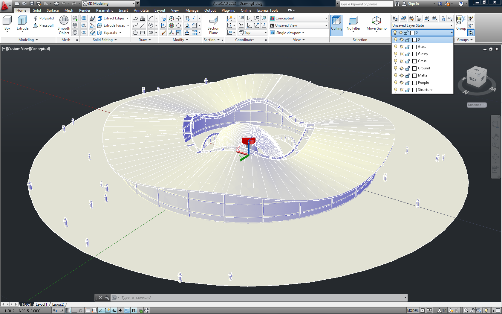
FIGURE ## | Model in AutoCAD with all the created layers.

To create a new material in AutoCAD, click the “Materials Browser” on the “Render” tab in the Ribbon, or write materials in the command line. The material browser should open.

FIGURE ## | FIGURE ## | View of the Material Browser.

In the Material Browser you should see, on the bottom part, a list of materials that come pre-installed with AutoCAD (if you chose the option to install them when you first installed AutoCAD) and, on the bottom, you will see a single material with the name “Global”. This is the default material that is loaded and applied to all the geometry in your model. You can choose a material from the pre-installed library if you want but for this example let’s create our own materials instead.

We will start with the material for the “Matte” layer to which we will be assigning a slightly white material with a matte finish. Click the “Create a New Material” button at the bottom of the Material Browser and select “New Generic Material”. A new generic material should appear on top of the material browser, above the existing Global material, and the corresponding material panel should appear on the side.

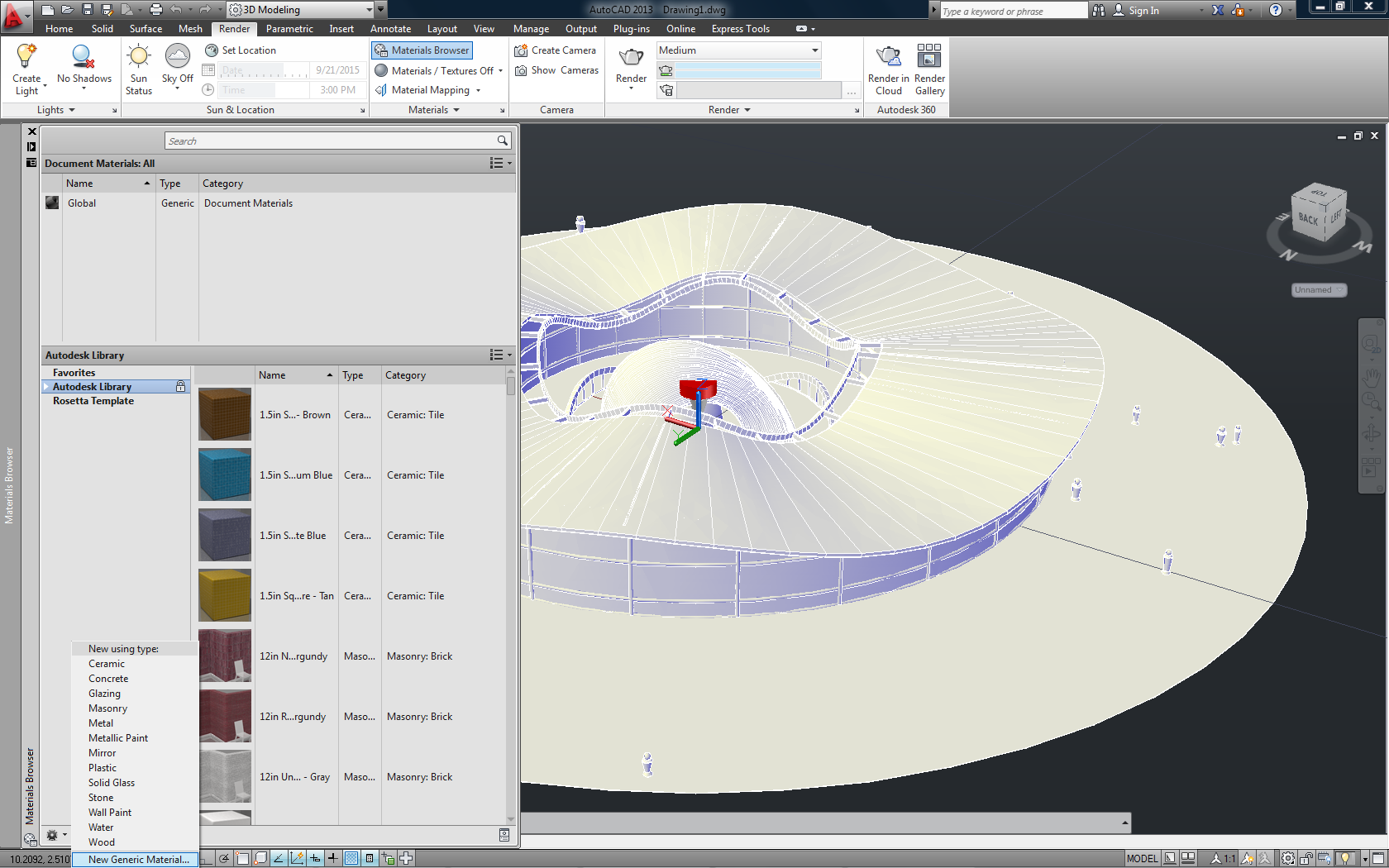
FIGURE ## | Creating a new generic material.

Let’s focus our attention on the Material Panel that came up. Click where it says “Default Generic” and rename this material to “White (Matte)”. Next, change the material colour from the default dark grey to a whitish colour (we recommend a material with a RGB value of 237,232,217) and move the “Glossiness” slider all the way down.

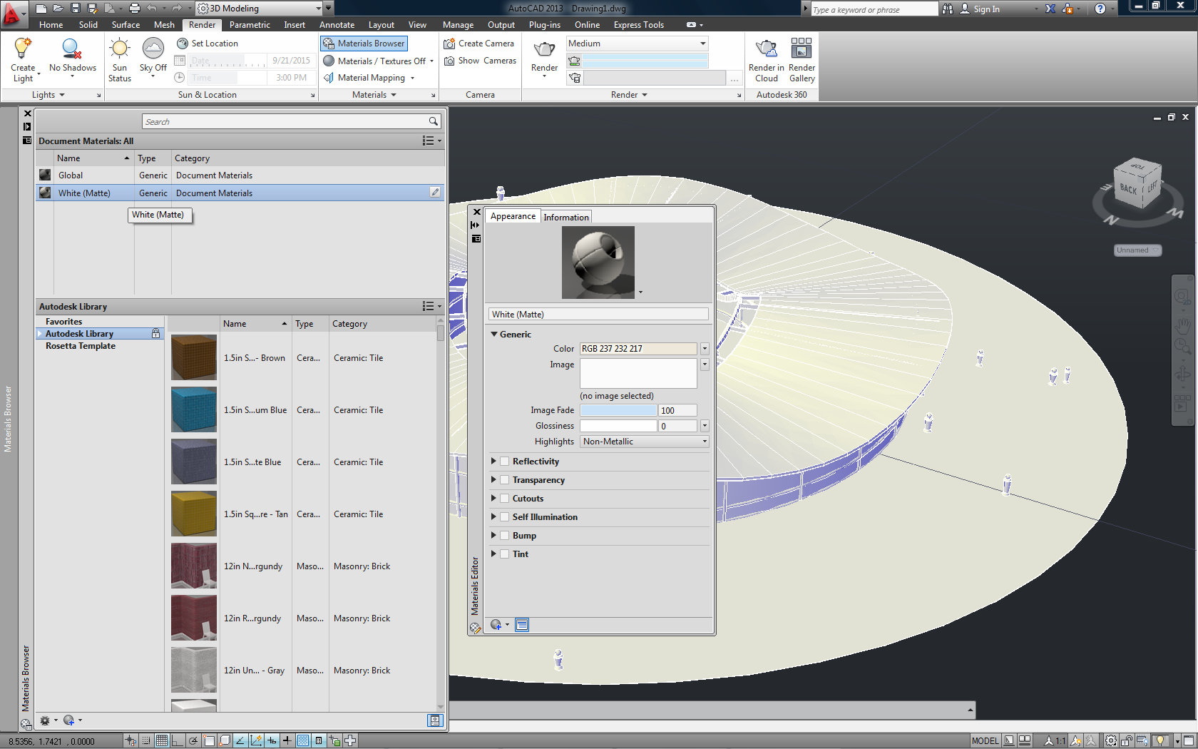
FIGURE ## | Changing the properties of the created generic material.

Close the material panel and let’s create the material for the “Glossy” layer. Create a new generic material as before, change its name to “White (Glossy)”, set the colour to the same whitish material but this time drag the “Glossiness” slider all the way up. Next, activate the “Reflectivity” option. Leave the “Direct” and “Oblique” values as they are but if you wish the material to be more or less reflective you can change these values at any time. Close this material panel.

FIGURE ## | Creating a glossy material.

For the “Structure” layer we want to create another generic material with the same properties as the “White (Matte)” material but give it a brownish colour to resemble a wood material. An alternative way to create a new material is to create a duplicate of an existing material and change its properties. Right-click over the “White (Matte)” material and choose “Duplicate”. A copy of that material will be created. Change its name to “Structure” and the colour to dark brown.

For the “Ground” layer we want to create a material with the same properties as the “White (Glossy”) but with a dark grey colour. Create a duplicate of the “White (Glossy)” material, change its name to “Ground” and the colour to a dark grey tone and set the reflection values to 60 (Direct) and 75 (Oblique).

Another material we need to create is for the “People” layer and in order to add some contrast let’s assign it a matte material with a strong red tone. Either create a new material or duplicate an existing one, name it “People” and choose a strong red colour.

The materials we have created so far are but generic materials to which we haven’t made any significant changes. For the remaining two layers “Glass” and “Grass” let’s do something a little different. In the “Material Browser” create a new material and instead of choosing “New Generic Material” choose instead “Solid Glass”. Name this new material “Glass”, give it a very light greenish tone (for example 221,232,221) and change the “Reflectance” value to 20. Leave the rest as it is.

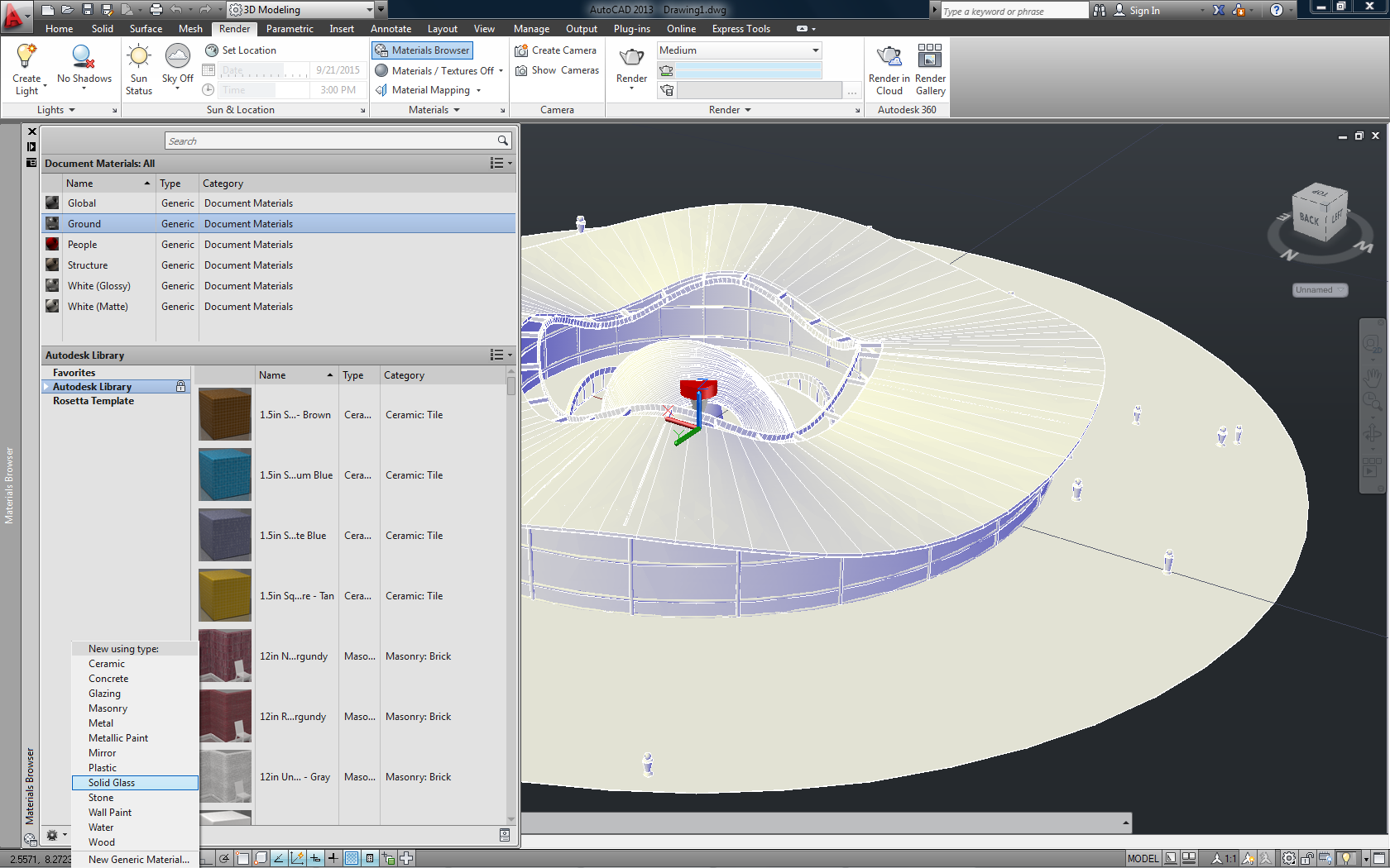
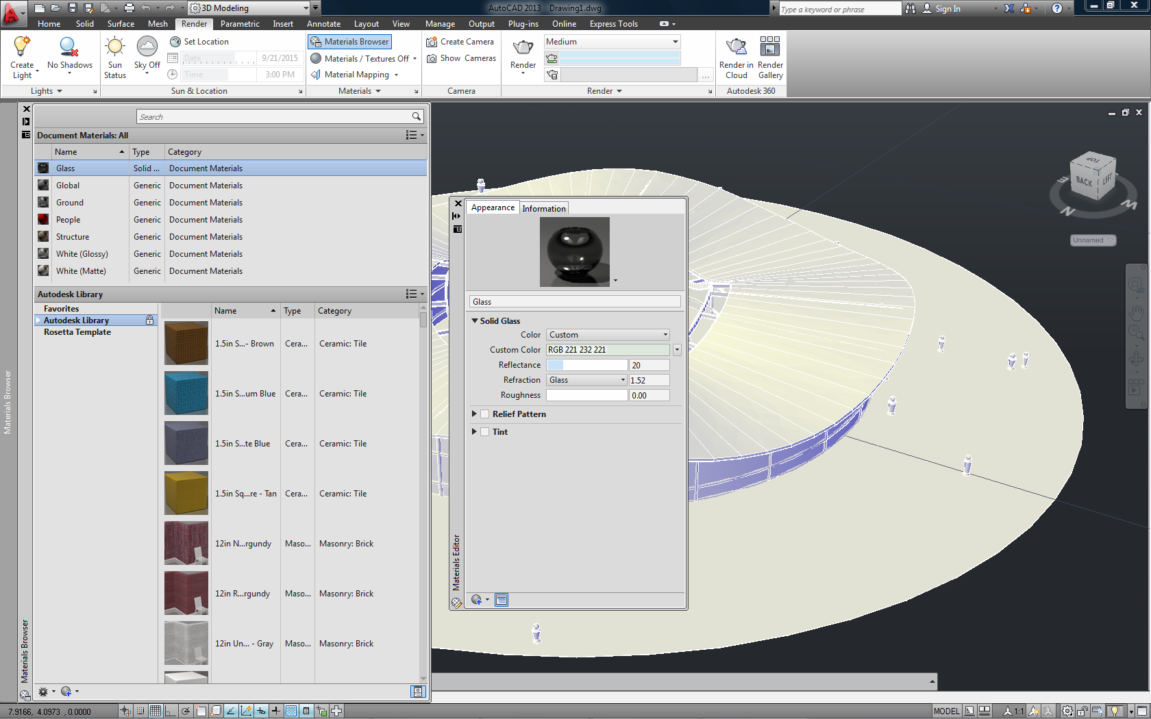
FIGURE ## | Creating a glossy material.

For the grass we will create a generic material but assign to it a texture. Create a Generic material and name it “Grass”. In the material tab, click the blank area next to “Image” and choose a grass texture. You can find several of them on the internet or in the pre-installed material library of AutoCAD. Click the loaded texture and a new tab will appear with some more texture settings. Change the scale size to 1 and remove the glossy finish.

(Most of these settings depend heavily on the scale of the model and textures being used. Therefore, keep in mind that you might need to try out different adjustments for your own case or in other models.)

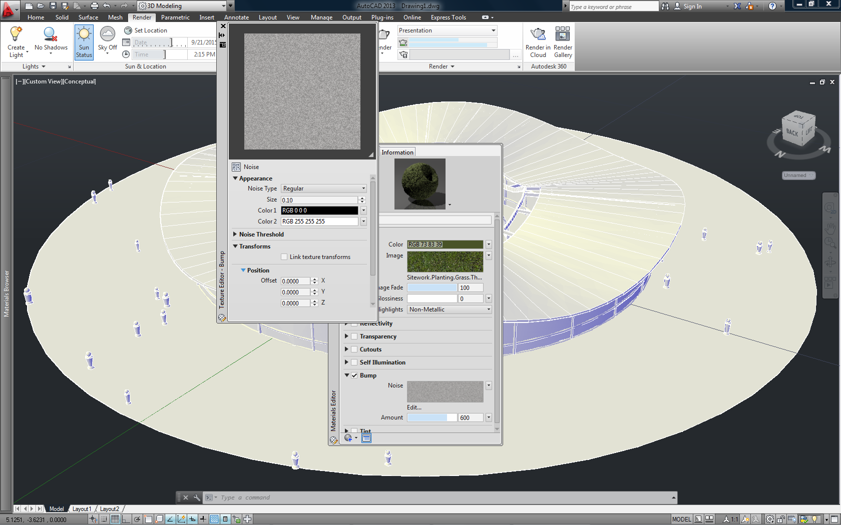
FIGURE ## | A grass textured material.

By now we have all the materials we need so now we want to assign them to their respective layer. To do this write in the command line materialattach. The Material Attachment Options window should pop up showing on the left side the materials we have created and on the left the layers we have in our document. All we need to do is drag and drop each material to the respective layer. When a material is assigned to a layer you should see a red cross next to the layer name, indicating there is a material assigned to that layer. If you click the cross the material will be removed.

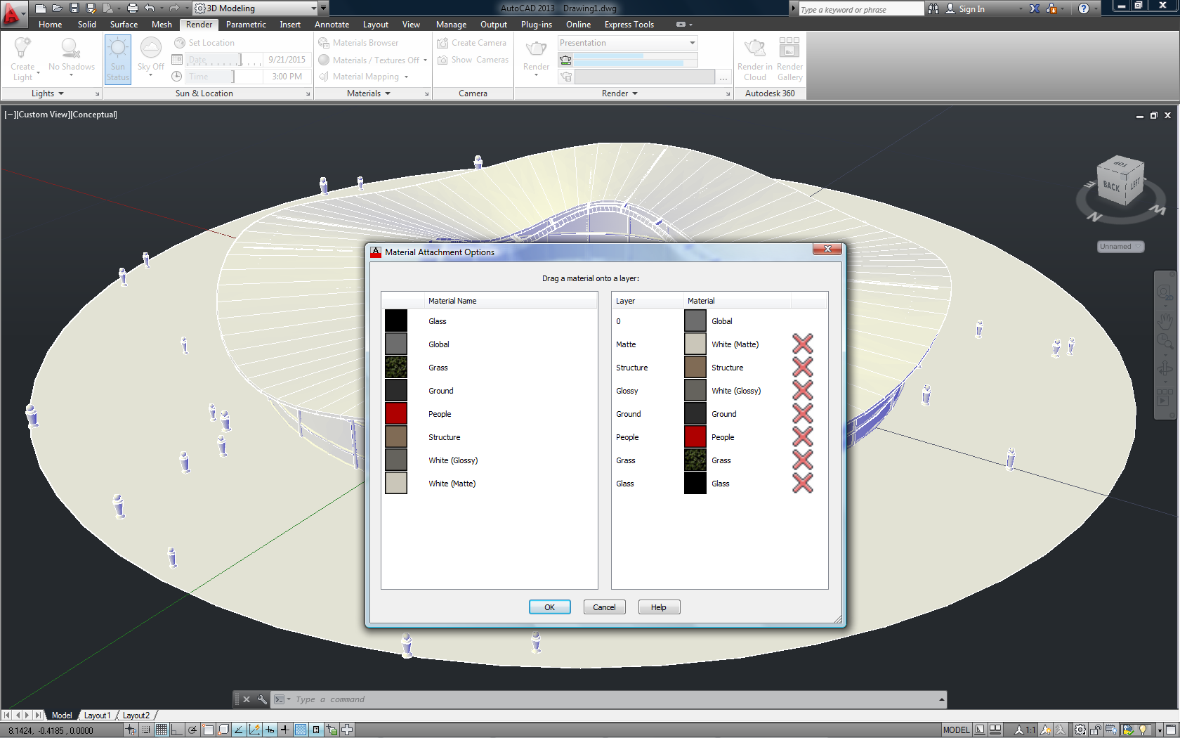
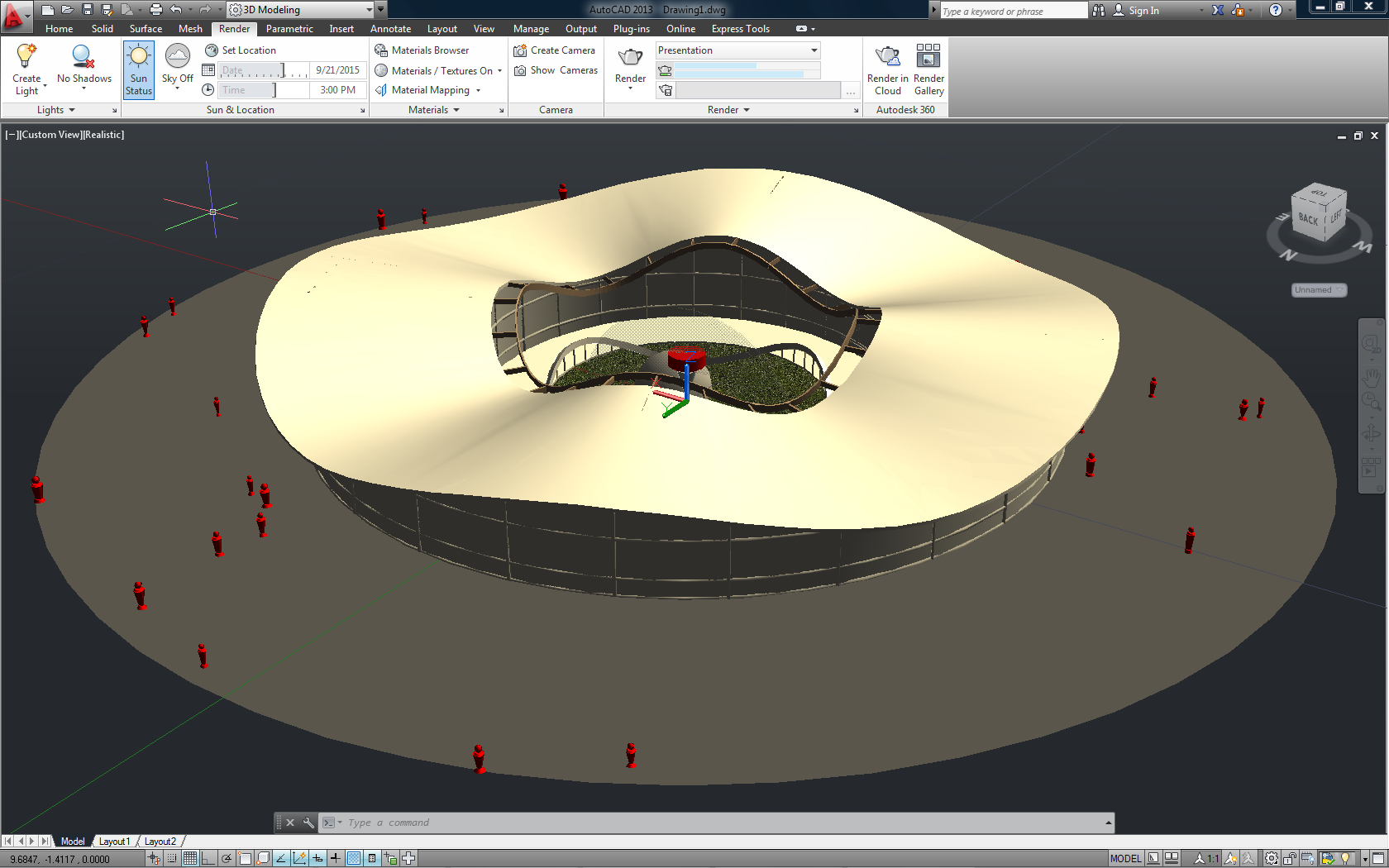
FIGURE ## | Assigning materials to layers.

We’ve completed the first prepping-up stage and if you have the visual style set to “Realistic” you should see each geometry with the assigned material. Let’s move on to configuring the render settings.

The first thing we want to do is, on the “Render” tab, click the “Sky Off” button and select “Sky Background and Illumination” instead. Alternatively write skystatus on the command line, write “2” and hit “Enter”. This will turn on the sun light and activate the environment properties. With the sun and environment turned one let’s go ahead and configure them.

Write sunproperties in the command line to bring up the Sun Properties tab, or click the small arrow on the bottom left corner of the “Sun & Location” tab in the Ribbon. Here we need to make sure the “General Status” is set to “On” and the “Sky Status” is set to “Sky Background and Illumination”. Give the Disk Scale a value of 10 and change the Intensity to 1.5. Under the “Sun Angle Calculator” tab choose your desired date and time (we recommend sometime between 12:00 and 15:00 for best results for a day render) and turn on “Daylight Saving”. The last change we will make is, under “Rendered Shadow Detail”, change the “Softness” value to “2”. If you want you can also change the geographic location for a more accurate sun angle calculation. You can do this by clicking the “Set Location” button at the “Sun & Location” tab in the Ribbon and either import geographic data, import geographic data from Google Earth or set the location manually. The process for doing this is pretty straightforward so we won’t show it in detail here.

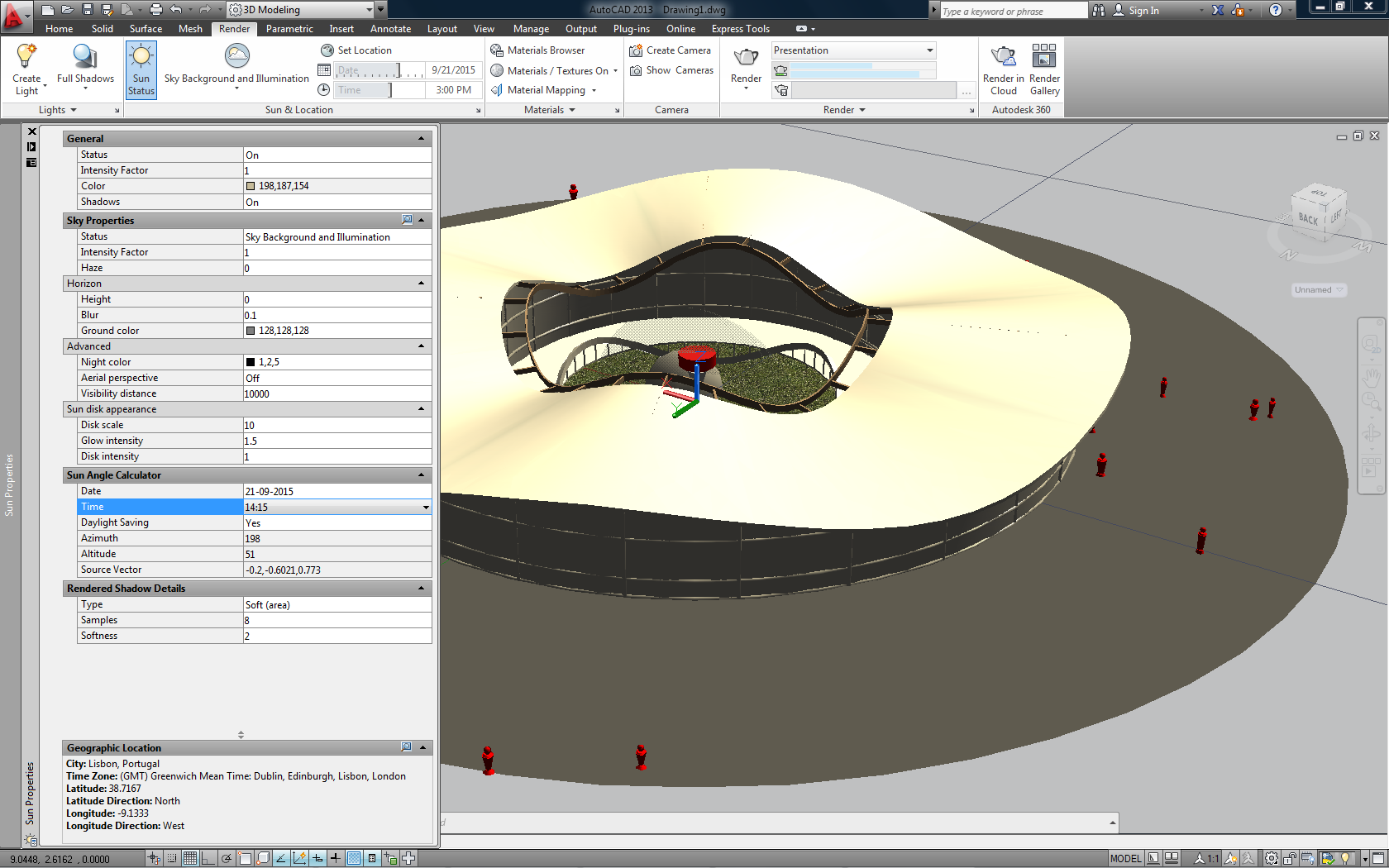
FIGURE ## | Sun and sky properties.

Moving on to the render properties. Either write rpref in the command line or click the small arrow on the corner of the “Render” tab in the Ribbon to bring up the “Advanced Render Options” tab. Here we can set a series of settings for the render but the most important of all is to turn “Global Illumination” on by clicking the light bulb next to it. On the top, in the “General” tab, you can also set other important settings such as the output size for you render. Choose a resolution of 1024x768 or manually input another resolution. On the very top of the “Advanced Render Options” panel there’s a dropdown menu for setting the overall quality of the render. By default it should be set to “Medium”. Change this to “Presentation” to get the best quality possible.

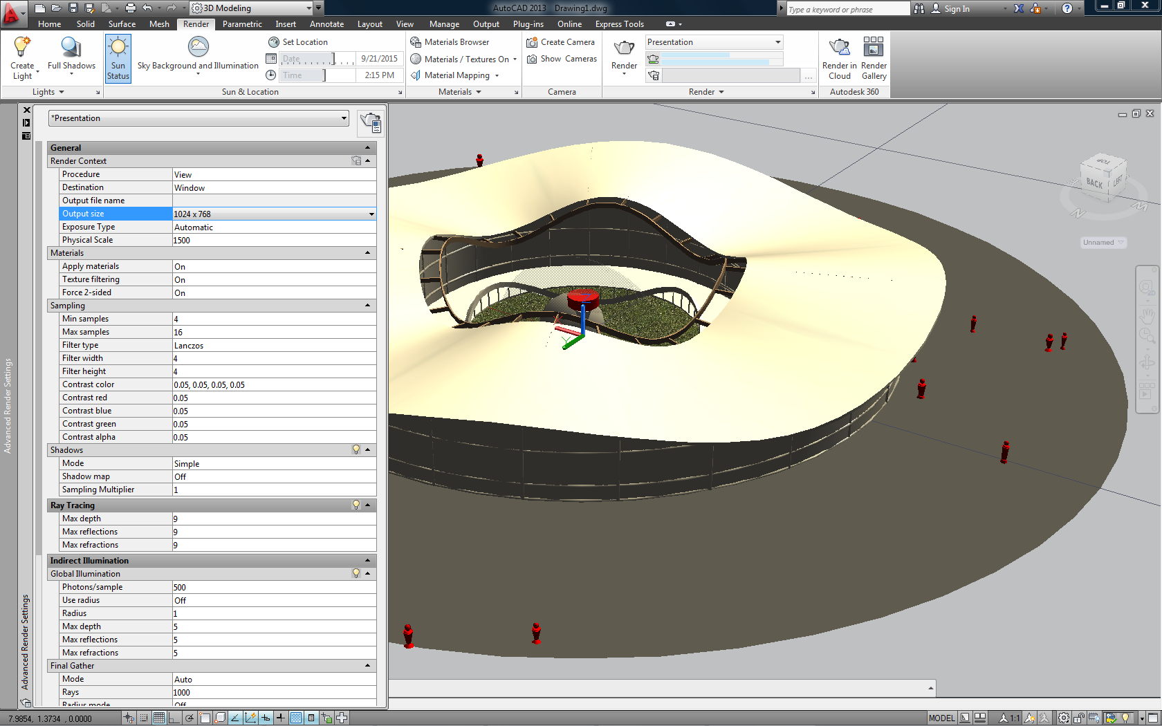
FIGURE ## | Advanced Render Properties.

Next we will adjust the Exposure Levels. This can be done by clicking the dropdown arrow in the Render tab and selecting Adjust Exposure” or by writing in the command line renderexposure. You should see a window pop where you can adjust the values of three parameters: Brightness, Contrast and Mid Tones.

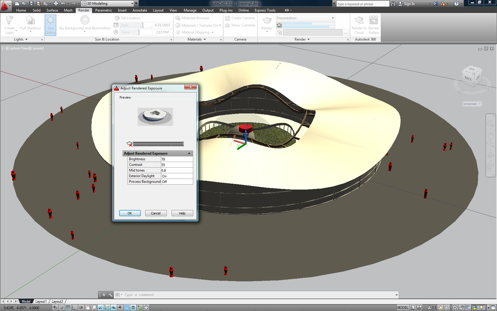
FIGURE ## | Adjust Rendered Exposure window.

The Brightness parameter controls the “White” of the final output render. The higher the value the more exposed the render will look. The Contrast parameter controls the “Black” levels and will enhance or decrease the dark areas in your render. The “Mid Tone” affects the ”Grey” values of the render. There are no concrete values here so you should play around to get the desired result. You can see the changes being applied on the small preview window. Based on experience we recommend “Brightness” values between 75 and 80, “Contrast” values between 52 and 55 and “Mid Tone” values between 0.8 and 1.0. Once you’re happy with how the preview looks click OK to set the exposure values.

We are now ready to render our model. Click the render button on the Render tab or write render in the command line to start the rendering process. You should see a window with your render being processed.

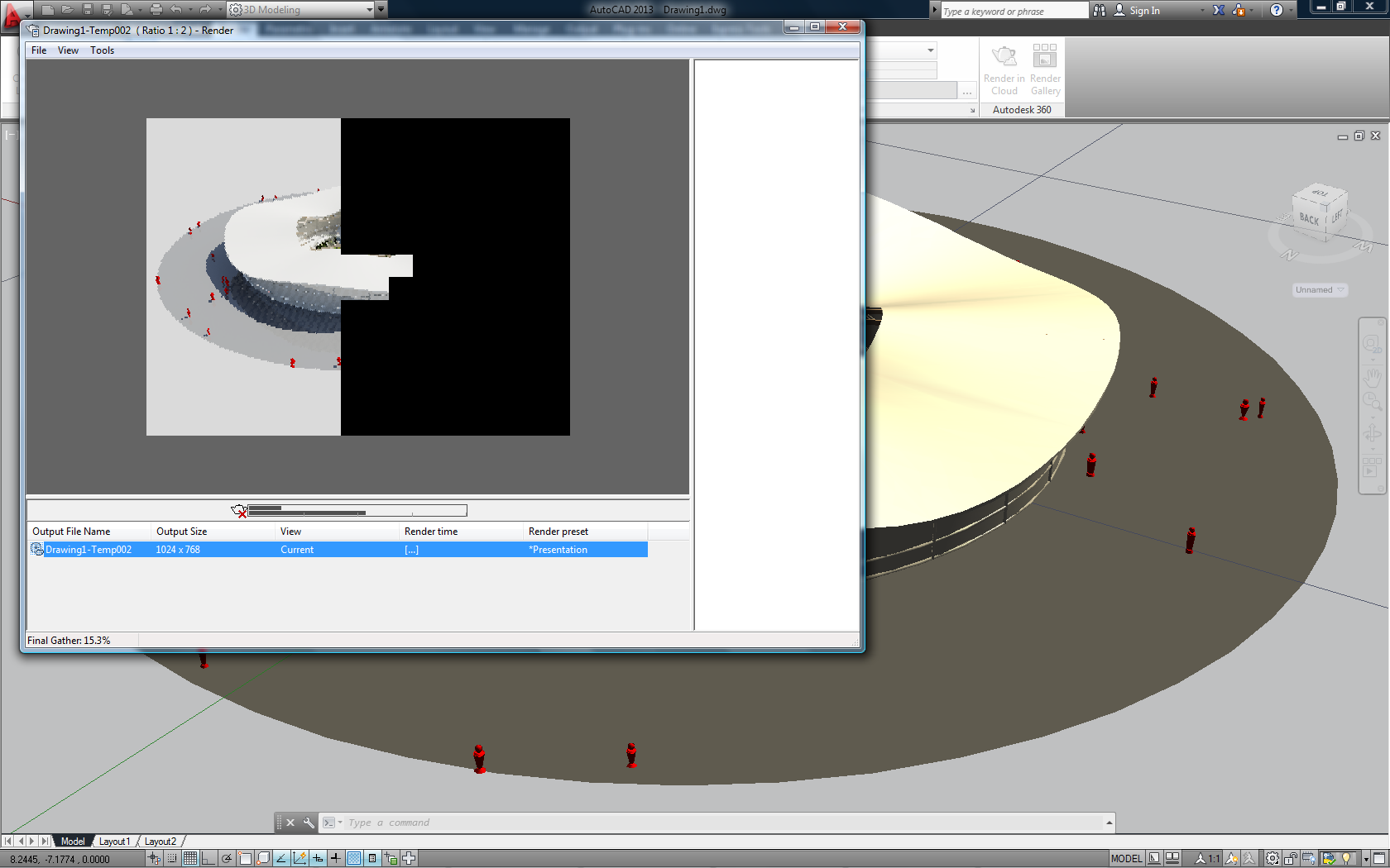
FIGURE ## | Render being processed.

Once the render is finish, and if we’re happy with the results, we need to save it. Right-click over the name of the render and choose “Save Copy”. Choose the destination folder where you wish to save the render and select the desired file type. If the render didn’t come out properly, if parts are too over exposed or the materials aren’t to our liking, then we should go back and change some settings to correct all the problems.

If you wish to save the render with the Alpha Channel, i.e., with transparency information for later compositing or post-processing, you need to save the image as either PNG, TIF or TGA. When you render an image there are parts of you render that are “drawn” – the actual model – and others – the background or transparent materials – that aren’t or are at least only partially drawn. This information is stored as an extra Alpha Channel (in addition to the RGB channels) and can be manipulated and applied to your render using an image editing software such as GIMP or Photoshop. Only certain file types support this transparency information though.

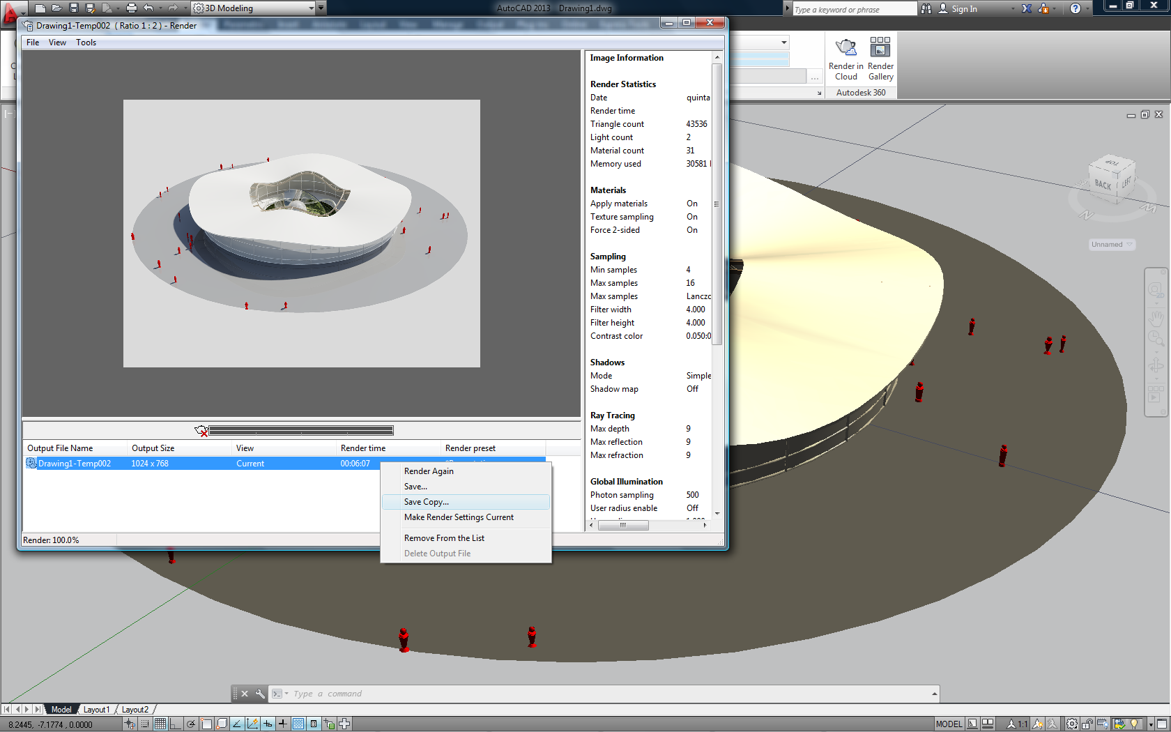
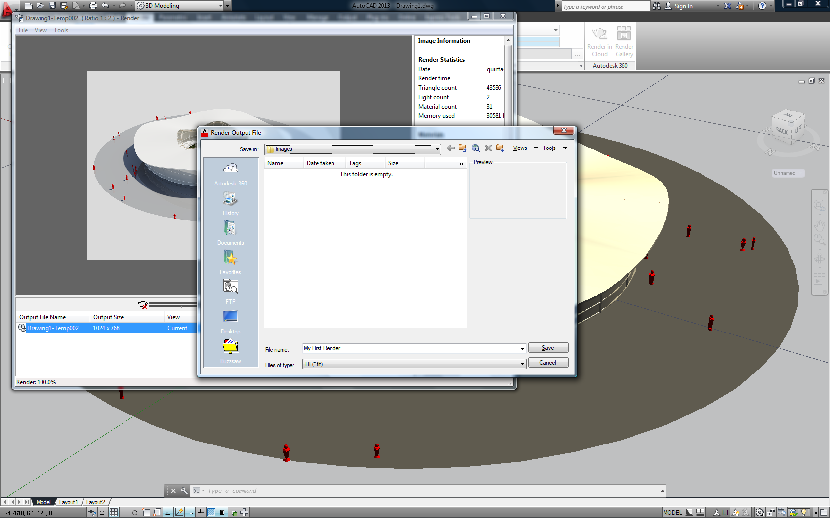
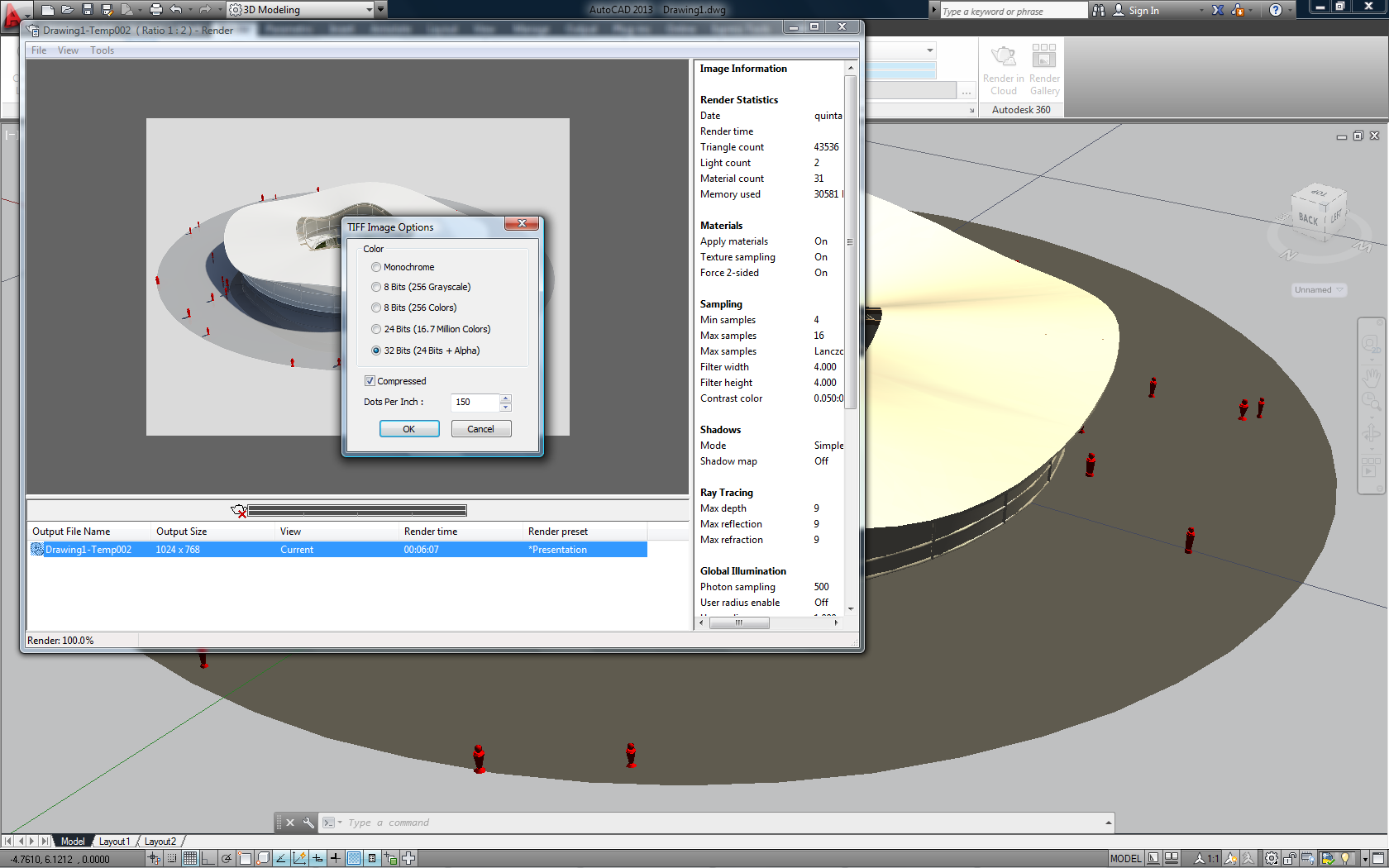
FIGURE ## | Saving the final output.

As we mentioned before, after you’ve done all the setting up you can also render with Rosetta by using the functions render-dir for specifying the save destination, render-size for setting the render resolution and render-view for performing the render. In Figure ## we can see three rendered images of our small building.

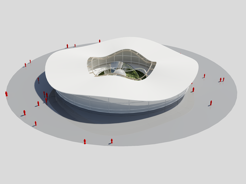
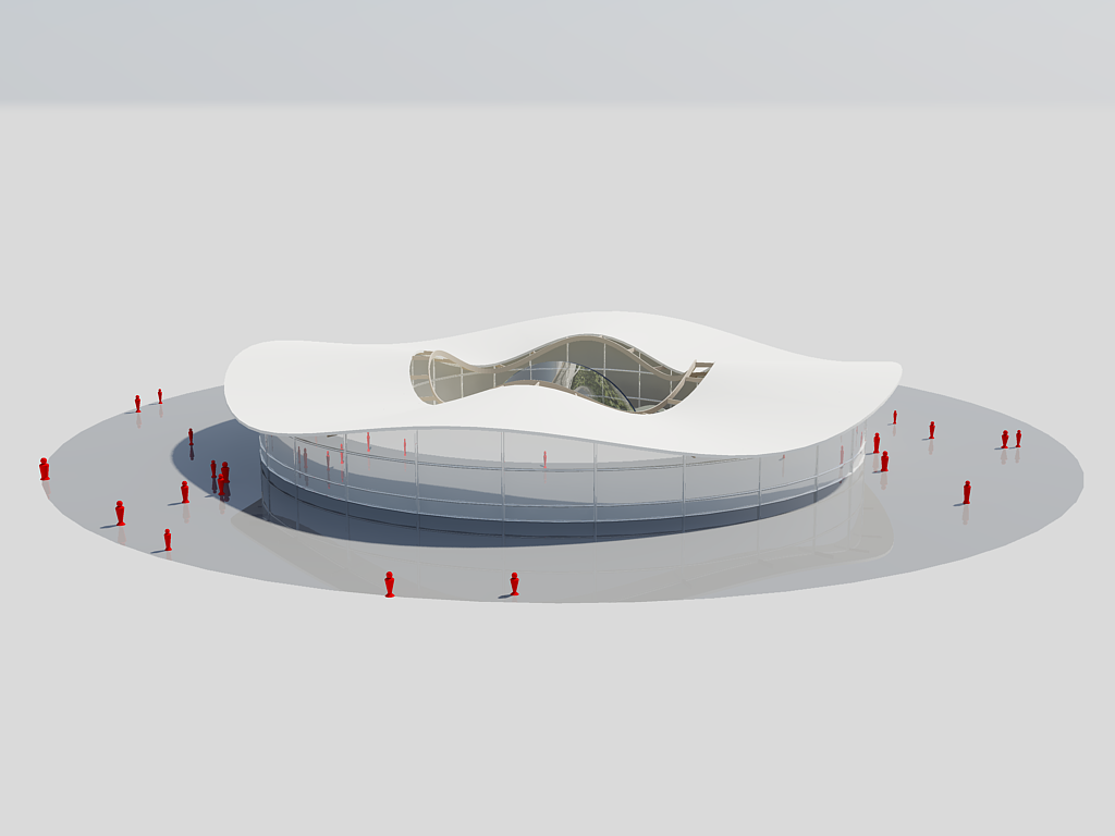
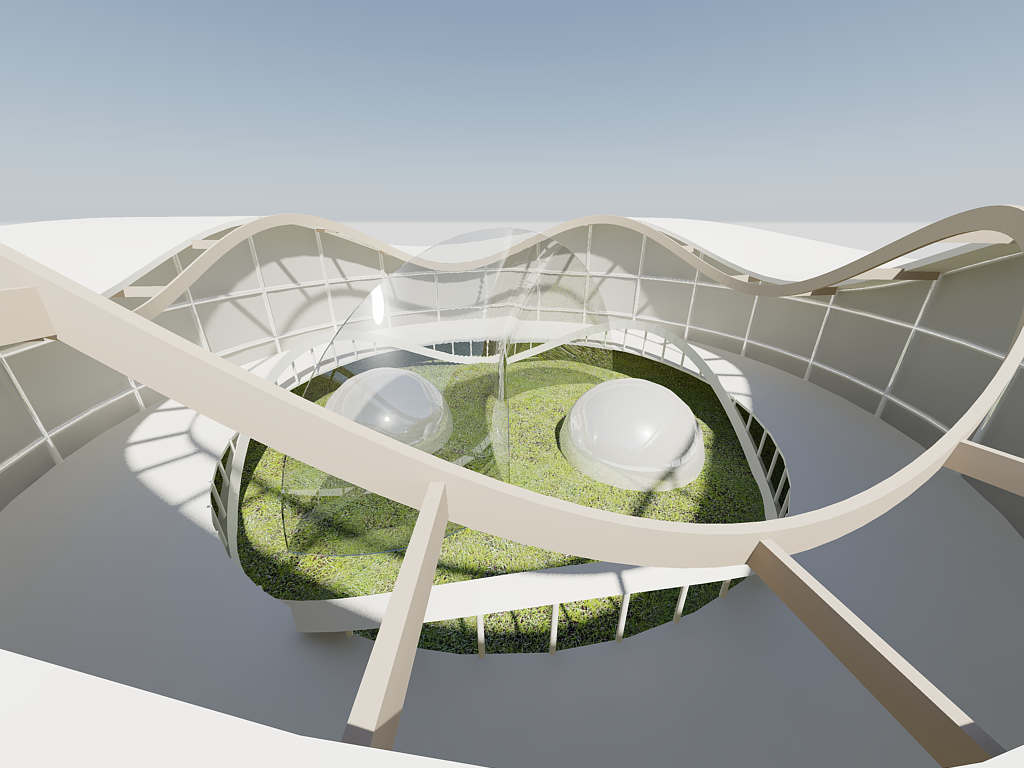
FIGURE ## | Three renders of our model from different points of view.

Producing a rendered image of our models is a good way of showcasing it and its features (shape, materials, environment, etc.) but what a render cannot be is dynamic. What you see in a render is what was generated with particular parameters and everything is fixed and static. If instead we wanted to show a particular feature of our model changing over time we would have our hands tied. This is where animations are useful.

Besides making renders Rosetta is also equipped with functions for making animations. Making an animation with Rosetta is nothing more than programming a sequence of renders to be performed one after the other, each render corresponding to one frame of the final animation. You can then take all the generated frames and create an animation from them. You can use animations for a series of purposes such as making flythroughs of your models or seeing parameters change over time.

The process of producing an animation is somewhat similar to producing a render. The first thing you need to take into consideration is the setting up of the template for the final output, which includes positioning the camera (using the combination of view-expression and view ), creating layers (with with-current-layer ), creating materials, assigning the materials to the layers and adjusting the sun, environment and render settings. Once all those things are done you can proceed with rendering the animation.

For programming an animation we will need to use two functions: start-film and save-film-frame . The start-film function tells Racket when it is supposed to start “recording” and this function is usually placed immediately before the invocation that generates our model. The save-film-frame , works similarly to render-view , and saves one frame of the film in a specific destination path and with the specified resolution. This function is placed inside the expression that generates the model. Remember that for setting the destination path you use render-dir and for setting the resolution you use render-size .

But let’s see how to do this with a concrete example. Suppose we have the model of a torus with a series of panels with openings along its surface. We will want to produce three animations:

• In the first animation we will simply have the parameter that affects the panel opening change over time. The animation should then show the panels opening and closing during the animation. The camera will be fixed and focusing on the torus;
• In the second animation we will have the openings being controlled by the distance to an attractor (represented with a small sphere) and have that attractor move around the torus. The camera will remain fixed and focused on the torus;
• In the third and final animation we will have the same things happening as in the second animation but the camera will follow and be focusing on the attractor.

It is very difficult, if not downright impossible, to create a template that works for every case possible. The settings we used in this tutorial might work well with the examples we’ve show but that is because there was some testing done beforehand to reach the results we wanted. Another model, with different geometry, different materials, different levels of detail and complexity, would probably require different settings to produce a good quality render. We thus encourage you to do some experimentation yourself.

It was also not the purpose of this tutorial to cover every little aspect of rendering in AutoCAD or Rhino but merely to show you how to do a basic setting up and how to render a model using Rosetta and Racket. For more information on this subject you can find several guides and tutorial on the internet. A good place to start would be the official documentation of AutoCAD and Rhino which you can find on their official webpage:

Autodesk Support page
Official Rhino3D tutorials