Additive Groves
The Additive Groves pointwise method, introduced by Sorokina et. al (2007), builds a ranking model through the formalisms of additive models and regression trees, attempting to directly minimize the training errors over the dataset.
In this approach, a grove is an additive model containing a small number of large trees. The ranking model of a grove is built upon the sum of the ranking models of each one of those trees.
The basic idea of Additive Groves is to initialize a grove with a single small tree. Iteratively, the grove is gradually expanded by adding a new tree or enlarging the existing trees of the model. The trees in the grove are then trained with the set of experts which were misclassified by the other previously trained trees. In addition, trees are discarded and retrained in turn until the overall predictions converge to a stable function. The goal of this algorithm is to find the simplest model which can make the most accurate predictions. The prediction of a grove is given by the sum of the predictions of the trees contained in it.
Additive Groves receives as input the parameter N, which is the number of trees in the grove, the parameter Α, which controls the size of each individual tree and the parameter b which is the number of bagging iterations, i.e. the number of additive models combined in the final ensemble. Algorithm 2, describes the Additive Groves algorithm proposed by Sorokina et. al (2007).
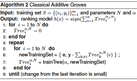
Following Algorithm 2, the first tree in the grove is trained using the entire original dataset, given by a set of pairs (e, y) (where e is an expert and $y$ is its respective relevance judgement). Supposing that T1 is the model computed by the first tree, then the next tree to be trained will focus only in the examination of the prediction errors of T1, in order to build a new ranking model which is able to classify elements intractable by the previous model. The algorithm continues this way until the root of the mean squares error can no longer be improved. The final model is given by simply combining all the models computed in all trees of the grove.
Since a single grove can easily suffer from overfit when the trees start to become very large, the authors introduced the bagging procedure to the model in order to overcome overfitting. Bagging is a method which reduces a model's performance by reducing variance. On each bagging iteration, the algorithm takes a bootstrap sample from the training set, and uses it to train the full model of the grove. When repeating this procedure a number of times, the algorithm ends up with an ensemble of models. The final prediction of the ensemble on each test data point is an average of the predictions of all models (Sorokina et. al, 2007).
Example of Application Additive Groves
If you want to test the Additive Groves algorithm, you should first download the Learning2Rank toolbox in GibHub.
This toolbox contains test datasets where you can run the algorithms and test them.
First, it is important to mention how the dataset files are structured. Each line of the file is a feature vector representation of the object that one wants to classify (for more information about how a learning to rank framework works, please check this section.
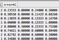
In the folder example_dataset/SmallAG/FoldX you can find two files in each Fold folder: trainAG and testAG. The trainAG file is the file that will be used by the algorithm to learn a function that is able to represent the data. On the other hand, the testAG file corresponds to examples that have not been learned by the algorithm. So, this file will be used to teste how good the learned function is.
The training and test data have the following format: classification feature1 feature2 ... featureN
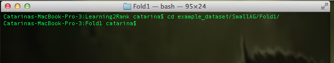
The first thing you should do is to open the terminal in the folder example_datasets/SmallAG/Fold1/. Note that we are going to perform a 4-fold cross validation. So, there are 4 fold folders that you must train. In this tutorial we will only show you how to train Fold 1. You must repeat the process for the remaining 3 folds.
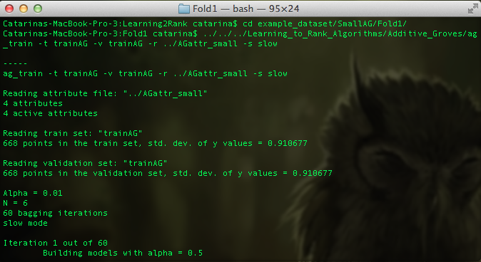
To train your dataset using the additive groves algorithm, open a command line terminal in the main folder of the Learning2Rank Toolbox and type the following command:
./Learning_to_Rank_Algorithms/Additive_Groves/ag_train -t _train_set_ -v _validation_set_ -r _attr_file_ [-a _alpha_value_] [-n _N_value_] [-b _bagging_iterations_] [-s slow|fast|layered] [-i _init_random_] [-c rms|roc]
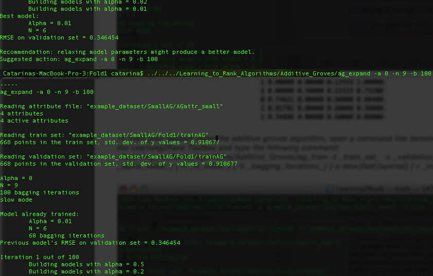
It can also happen that you need to relax a little your training model, so the algorithm will suggest you to set some parameters:
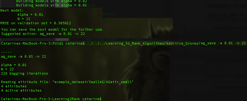
When the algorithm finishes the training process, it will ask you to save the model. You just need to type ag_save [-n n_param] [-a a_param].
There should be a new file model.bin inside the FoldX folder that you are training. This file corresponds to the model learned by the machine learning algorithm.
To test your dataset using the additive groves algorithm, open a command line terminal in the main folder of the Learning2Rank Toolbox and type the following command:
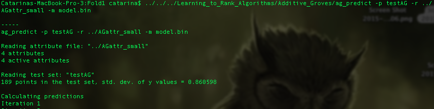
./Learning_to_Rank_Algorithms/Additive_Groves/ag_predict -p _test_set_ -r _attr_file_name_ [-m _model_file_name_] [-o _output_file_name_] [-c rms|roc]
This command will generate a prediction file that corresponds to the predictions that the trained model.bin achieved for each single feature vector of the file testAG.
Since we are training with a 4-fold cross validation method, you need to repeat the training for the remaining 3 folds. When this is finished, and after having the prediction files from the 4 folds, then we can evaluate our model.
In the Learning2Rank toolbox, it is provided an executable file that evaluates how good the trained model is over the test data. What this does is simple: for each query, the program is going to check how many objects it classified correctly. To know this information, first you need to place the terminal in the directory where the file generate_trec_eval.jar is. Then, you just need to run the following command:
java -jar generate-treceval-files.jar example_dataset/SmallAG/ MAP 4

For this example, we achieved a Mean Average Precision (MAP) of 0.7454. The executable generate-treceval-files.jar will generate three additional files: qRel, qResults and results.
- qRel: contains the relevance judgements of each feature vector contained in the prediction file.
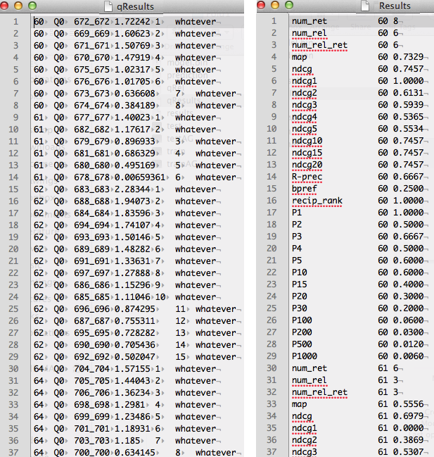
- qResults: for each feature vector in the prediction file, it contains the ranking for each query and the relevance judgement.
- results: contains the evaluation for severa metrics for each query. In the end, it contains the average over all queries for the different evaluation metrics.