5.4 Urban Design
Cities are a good example of the combination between regularity and randomness. Although many ancient cities appear to be chaotic, as a result of their unplanned development, others already encompassed a structured plan, in order to facilitate their growth and improve their living environment. In fact, there are well-known examples of planed cities dating from 2600 BC.
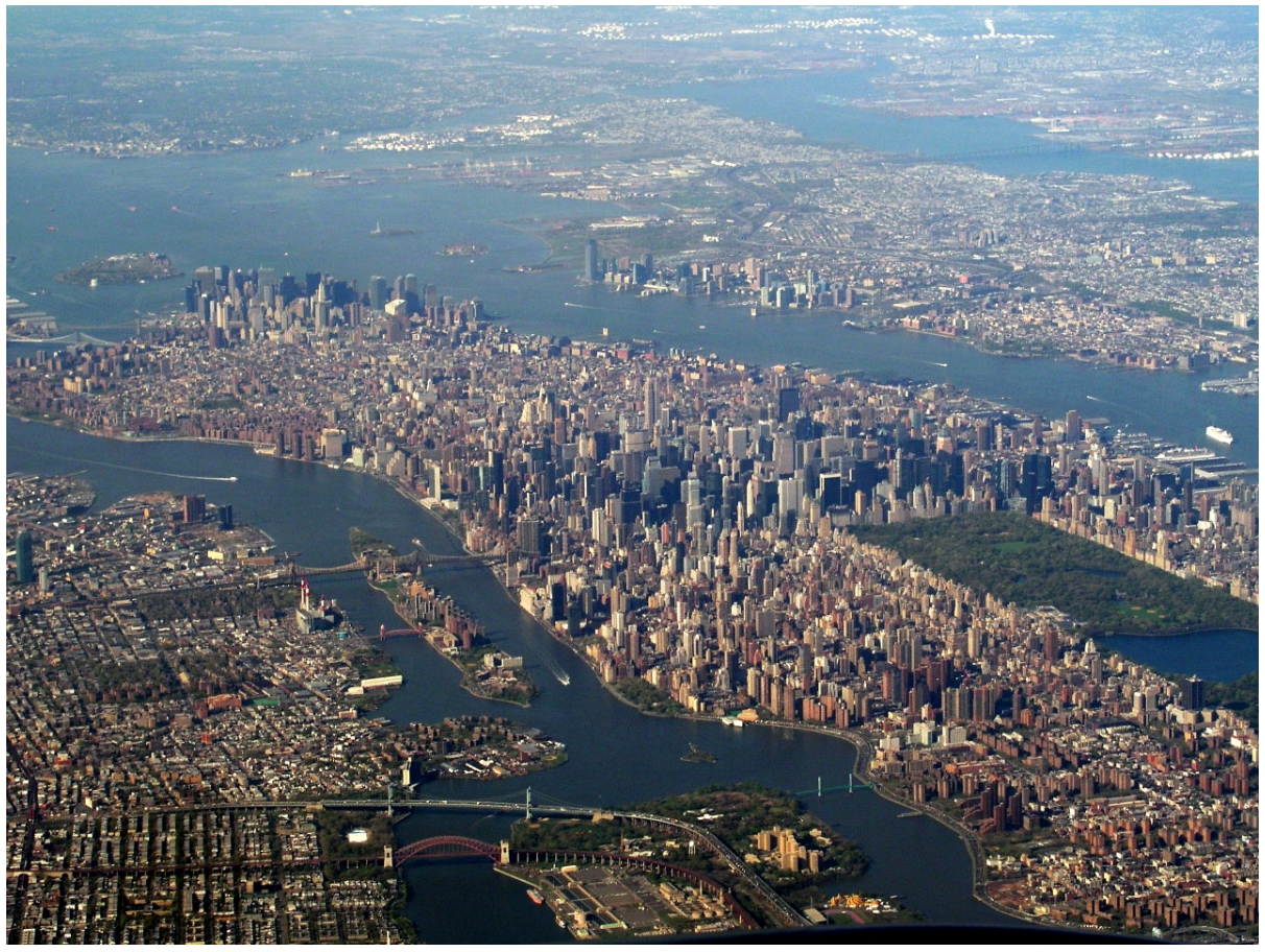
Despite the variety of approaches, the two most usual ways of planning a city are through the orthogonal plan or the circular plan. In the orthogonal plan, straight streets make right angles between them. In the circular plan, the main streets are radial, converging into a central square, whereas the secondary streets are concentric circles around this main square, following the city’s growth. In this section we will explore randomness to simulate cities that follow an orthogonal plan. A good example of a city mainly developed according to this plan is shown in this figure.
Aerial view of New York City. Photograph by Art Siegel.
In an orthogonal plan, the city is organized into blocks. Each block assumes a rectangular or square shape and contains several buildings. To simplify, we will assume that each block has a square shape with fixed size and contains a single building with a fixed height that occupies the entire block. The buildings are separated from each other by streets with a fixed width. The model of this city is presented in this figure.
Scheme of an orthogonal city plan.

In order to structure the function that creates a city with an orthogonal plan, we will first decompose the process into the construction of the successive rows of buildings. Then, the construction of each row of buildings is further decomposed in the successive construction of buildings. Thus, we must parametrize the function based on the number of rows and on the number of buildings per row. In addition, we will need to know the city’s origin point \(P\), the length \(l\) and height \(h\) of each building, and, finally, the width \(s\) of each street. The function will first create a row of buildings separated by streets and then, recursively creates the rest of the city. To simplify this process, we will assume that streets are aligned with the \(X\) and \(Y\) axes, whereby each new row corresponds to a displacement along the \(Y\) axis and each new building corresponds to a displacement along the \(X\) axis. Thus, we will have:
city(p, n, m, l, h, s) =
if n == 0
nothing
else
buildings(p, m, l, h, s)
city(p + vy(l + s), n - 1, m, l, h, s)
end
For the construction of a row of buildings, the process is the same: we place a building at the starting location and, then, we recursively place the remaining buildings at the next location. The following function implements this process:
buildings(p, m, l, h, s) =
if m == 0
nothing
else
building(p, l, h)
buildings(p + vx(l + s), m - 1, l, h, s)
end
Finally, we need to define a function that creates a building. To simplify, we will model each building as a parallelepiped:
building(p, l, h) = box(p, l, l, h)
With these three functions we can now try to build a small city. For example, the following expression creates a set of ten rows of buildings with ten buildings per row:
city(xyz(0, 0, 0), 10, 10, 100, 400, 40)
The result is presented in this figure.
An urban area with an orthogonal plan, containing one hundred buildings with the same height.

However, the generated urbanization lacks some of the randomness that typically characterizes cities. To incorporate some randomness, we we will consider that the buildings’ height can randomly vary from a maximum height to one-tenth of that height. This behavior was implemented in a new definition of the building function:
building(p, l, h) = box(p, l, l, random_range(0.1, 1.0)*h)
Using the exact same parameters as before in two consecutive calls of the building function, we can now generate more appealing cities, as shown in this figure and this figure.
An urban area with an orthogonal plan, containing one hundred buildings with random heights.

An urban area with an orthogonal plan, containing one hundred buildings with random heights.

5.4.1 Exercises 28
5.4.1.1 Question 83
The cities produced by the previous functions do not present sufficient variability, as all the buildings have the same shape. To solve this issue, define different functions for different types of buildings: the building0 function should build a parallelepiped with random height (as before), and the building1 function should build a cylindrical tower with a random height (also varying from 10% to 100% of a maximum height), contained within the limits of a block. Then, use both building0 and building1 functions to redefine the building function, so that it randomly generates different buildings. The resulting city should be composed of \(20\%\) circular towers and \(80\%\) rectangular buildings, as illustrated in the following figure:

5.4.1.2 Question 84
The cities created in the previous exercise only allow the creation of two types of buildings: rectangular or cylindrical. However, when we observe a real city, as the one shown in this figure, we find out that there are buildings with many other shapes. This means that, in order to increase the realism of our simulated cities, we need to implement a larger number of functions, each one creating a different kind of building.
View of Manhattan. Photograph by James K. Poole.
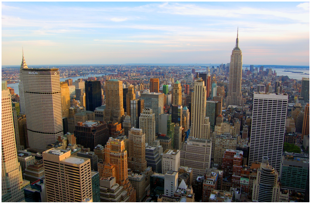
Fortunately, a careful observation of this figure shows that, in fact, many of the buildings follow a pattern that can be modeled by stacking successively smaller parallelepipeds with random dimensions. This is something that we can easily implement with a single function.
Consider that such buildings are parametrized by the number of intended blocks to stack, the coordinates of the first block and the length, width and height of the building. The base block has exactly the specified length and width but its height should range between \(20\%\) and \(80\%\) of the total height. The remaining blocks are centered on the block immediately below, with a length and width ranging between \(70\%\) and \(100\%\) of the corresponding parameters of the block immediately below. The height of these blocks should range between \(20\%\) and \(80\%\) of the remaining height of the building. The following image shows some examples of buildings that follow this model:

Based on this specification, define the building_blocks function and use it to redefine the building0 function, so that the generated buildings have a random number of stacking blocks, ranging between \(1\) and \(6\). With this redefinition, the city function should be able to generate a model similar to the following image:

5.4.1.3 Question 85
Typically, cities have an area of relatively tall buildings, which is called business center (abbreviated to CBD, an acronym of Central Business District). As we move away from this area, the height of the buildings tends to decrease, as is visible in this figure.
The variation of the buildings height can be modeled by several mathematical functions but, in this exercise, we intent to apply the two-dimensional Gaussian distribution, given by:
\[f(x,y) = e^{-\left( (\frac{x-x_o}{\sigma_x})^2 + (\frac{y-y_o}{\sigma_y})^2\right)}\]
In the previous formula, \(f\) is the weighting height factor, \((x_0\) and \(y_0)\) are the coordinates of the highest point of the Gaussian surface, and \(\sigma_0\) and \(\sigma_1\) are the factors that determinate the two-dimensional stretch of this surface. In order to simplify, assume that the highest point of the business center is located at the position \((0,0)\) and that \(\sigma_x=\sigma_y=25 l\), with \(l\) being the building’s length. The following image shows an example of one such city:

Incorporate this distribution in the city generation process to produce more realistic cities.
5.4.1.4 Question 86
Cities often have more than one center of tall buildings. These centers are separated from each other by zones of smaller buildings. As in the previous exercise, each area of buildings can be modeled by a Gaussian distribution. Assuming that the multiple areas are independent from each other, the buildings’ height can be controlled by the overlapping of Gaussian distributions, i.e., at each point, the buildings’ height is the maximum height of the Gaussian distributions of the different areas.
Use the previous approach to model a city with three areas of “skyscrapers”, similar to the one presented in the following image:

5.4.1.5 Question 87
It is intended to create a set of \(n\) tangent spheres to a virtual sphere centered at \(P\), with a limit radius \(r_l\). The spheres are centered at a random distance of \(P\), which corresponds to a random value between an inner radius \(r_i\) and an outer radius \(r_o\), as presented in the following scheme:

Define a function called spheres_in_sphere that, from the center \(P\), the radii \(r_i\), \(r_o\), and \(r_l\), and a number \(n\), creates a set of \(n\) spheres, similar to the ones in the following image:
