ROSETTA

Contents:
• Part I - Points and Curves
• Part II - Irregular and Regular Polygons
• Part III - Circles, Ellipses and Arcs
• Part IV - Surfaces

In the previous tutorial we saw how to use coordinate systems to specify positions in space. With that in mind we are now capable of starting actually creating geometry we can see in a CAD and in this tutorial we’ll glance over the primitive functions in Rosetta that allow you to do that. The first geometric primitive we’ll look at are points and curves and by curves we mean everything from lines, polygonal lines and splines, either open or closed.

For creating points Rosetta provides the function point. This function takes as arguments a single position in space specified in any desired coordinate system.

(point (xyz 2 3 0))
(point (pol 6 pi/3))

If we want to draw lines we can use the function line which receives either the position of the two extremity points or a list positions to interpolate the line through.

(line (xy 0 0) (xy 5 0) (xy 5 5) (xy 0 5) (xy 0 0))
(line (list (xy 0 0) (xy 5 0) (xy 5 5) (xy 0 5) (xy 0 0)))

FIGURE 1 | A set of line segments

The lines we are creating are straight polygonal line segments but it is often the case that we want to draw interpolated curves through a series of points. Using Rosetta’s spline function we can achieve this. Like the line function the spline function needs to receive a series of points either input individually or in the form of a list. We also have the option of using the function closed-spline if we want the spline to be automatically closed at the end. We can see in Figure 2 the result of the expression below. For the sake of clarity we have also included the points in this figure although they are not created by the function.

(spline (list (xy 0 2) (xy 1 4) (xy 2 0) (xy 3 3)
              (xy 5 0) (xy 5 4) (xy 6 0) (xy 7 2)
              (xy 8 1) (xy 9 4)))

FIGURE 2 | A spline interpolated through a series of points

You may have noticed that in previous example we had to repeat the last location (xyz 0 0 0) in order to close the shape we were creating. If we want to draw closed shapes then it’s much more convenient to use the functions polygon which works exactly the same way but automatically connects the last given position with the first one.

(closed-line (xy 0 0) (xy 5 0) (xy 5 5) (xy 0 5))

(polygon (pol 1 (* 2 pi 0/5)) (pol 1 (* 2 pi 1/5))
         (pol 1 (* 2 pi 2/5)) (pol 1 (* 2 pi 3/5))
         (pol 1 (* 2 pi 4/5)))

FIGURE 3 | Two closed polygons

The function polygon is therefore useful for creating irregular polygons with any number of sides. One very common type of irregular polygon is the rectangle. To draw one we could obviously use the function polygon and feed it the necessary positions but Rosetta provides a more direct way of creating rectangles with the function rectangle. To create a rectangle with this function we can specify the bottom-left corner, length and width of the rectangle or alternatively the bottom-left and top-right corners.

(rectangle (xy 0 0) 10 6)
(rectangle (xy 0 0) (xy 5 6))
(rectangle (xy 0 0) 5 3)
(rectangle (xy 0 0) (xy 2.5 3))
(rectangle (xy 0 0) 2.5 1.5)

FIGURE 4 | Rectangles created with different methods

We won’t always want to create irregular polygon. In fact changes are that we’ll need to create regular polygon more often than irregular ones. The function polygon is good for creating irregular polygons but to create regular polygons, the fact that we need to specify each vertex, makes it a painstakingly process. There is an easier way of creating regular polygons by using the regular-polygon function. This function creates a regular n-sided polygon inscribed or circumscribed in a circle. The user must specify the number of sides desired for the polygon, the circle’s centre point, radius and initial angle with the horizontal axis. We can also provide an additional parameter for specifying if the polygon is inscribed or circumscribed (#t for inscribed and #f for circumscribed).

(regular-polygon 3 (xy 0 0) 1 0 #t)
(regular-polygon 3 (xy 0 0) 1 (/ pi 3) #t)

(regular-polygon 4 (xy 3 0) 1 0 #t)
(regular-polygon 4 (xy 3 0) 1 (/ pi 4) #t)

(regular-polygon 5 (xy 6 0) 1 0 #t)
(regular-polygon 5 (xy 6 0) 1 (/ pi 5) #t)

FIGURE 5 | A set of regular polygons

Let’s now consider the creation of circles. Using the function circle we can specify a circle by its centre point and radius.

(circle (pol 0 0) 4)
(circle (pol 4 (/ pi 4)) 2)
(circle (pol 6 (/ pi 4)) 1)

FIGURE 6 | Three circles along a diagonal

Let’s exemplify this function with another exercise. Say we went to draw the first iteration of an Apollonian Gasket, a known fractal composed of tangent circles inscribed in a larger circle, as shown in Figure 7.

FIGURE 7 | The Apollonian Gasket. Source: Wikipedia

To model the first iteration of this fractal, without going into recursion, we need only use the circle function and, using simple trigonometry, calculate the three centre points that allow the tangency to occur. In Figure 7 we’ve identified an inner triangle and three variables – A is the distance from the centre point p to one of the circle’s centre point, B is the circle’s radius and C is the distance from p to one of the tangency points. Using trigonometry we can deduce that:

The nature of this exercise asks for us to use polar coordinates since we are working with radii, angles and circles. In Figure 7 we have also identified three additional variables – p0, p1 and p2 which are the centre points for our three circles. The location of them can be determined in terms of p, the distance A and an angle. Those angles are easily calculated by knowing that inner triangle has the angles 30º, 60º and 90º or better yet pi/6, pi/3 and or pi/2.

We only want our 3-tangent-circles function to have as parameters an insertion point p and the radius r of the three circles. All other variables (a, p0, p1, p2) should be set as local variables. A local variable is a variable which is only has meaning in the context of the function where it exists and is used to calculate intermediate values. When we define a function using Racket’s form define, that function remains active or “meaningful” throughout the entire program we are writing and we call that a global variable. A local variable will only affect the function it is in. To set local variables we use Racket’s let form or its variant let*. The difference from the two is that local variables set using let will be independent from each other while let* will set the variables in a dependent cascading sequence. Once the local variables are set we can use them in the body of our function like any other parameter.

Let’s then write the function 3-tangent-circles:

(define (3-tangent-circles p r)
  (let* ((a (* 2 (/ r (sqrt 3))))
         (p0 (+pol p a pi/2))
         (p1 (+pol p a (+ pi (/ (* 5 pi) 6))))
         (p2 (+pol p a (- (/ (* 5 pi) 6)))))
    (circle p (+ r a))
    (circle p0 r)
    (circle p1 r)
    (circle p2 r)))

If you look closely at the local variables being set you can see that the first local variable a also appears in the next ones. If we had used let instead of let* Racket would return an error saying a had not be defined. This is what we mean my setting variables in a dependent cascading sequence. In Figure 8 we can see the result of testing this function.

FIGURE 8 | Three tangent circles

If instead of circles we want to draw ellipses we can use the function ellipse specified by its centre point and major and minor radii. If both radii are equal obviously the result will be a circle.

(ellipse (xy 0 0) 10 5)
(ellipse (xy 0 0) 6 5)
(ellipse (xy 0 0) 3 5)
(ellipse (xy 0 0) 1 1)

FIGURE 9 | Concentrical ellipses

Lastly we might want to create arcs and for that Rosetta provides the function arc which creates a circular arc specified by its centre point and angle domains between which to draw the arc.

(arc (xy 0 0) 4 0 pi)
(arc (xy -2 0) 2 pi/2 pi/2)
(arc (xy 0 2) 2 -pi/2 -pi/2)

(arc (xy 8 0) 4 0 -pi/2)
(arc (xy 6 0) 6 0 -pi)
(arc (xy 4 -4) 4 0 pi/2)

FIGURE 10 | A series of circular arcs

Note that the second angle provided is in relation to the first one. So, if we define the domain [π/2,π/3] that means the arc will start at π/2 and to that π/3 will be added.

Many of these functions that create closed shapes also have an alternate version with the same parameters but which produce surfaces instead of lines or curves:

• • surface-rectangle
• • surface-circle
• • surface-polygon
• • surface-regular-polygon
• • surface-arc

One little comment should be made referring the last function surface-arc. An arc is obviously an open curve yet it can be made into a surface using that function. The result will be a “slice” or a sector of a circle. Bellow in Figure 11 we can see the difference result produced between the functions arc and surface-arc.

(arc (xy 0 0) 4 pi/6 (* 2 -pi/6))
(arc (xy 0 0) 4 (- pi pi/6) (* 2 pi/6))
(arc (xy 0 0) 2 pi/4 pi/2)
(arc (xy 0 0) 3 -pi/4 -pi/2)

(surface-arc (xy 10 0) 4 pi/6 (* 2 -pi/6))
(surface-arc (xy 10 0) 4 (- pi pi/6) (* 2 pi/6))
(surface-arc (xy 10 0) 2 pi/4 pi/2)
(surface-arc (xy 10 0) 3 -pi/4 -pi/2)

FIGURE 11 | Difference between arc and arc-surface

All the other functions are pretty straightforward.

(rectangle (xy 0 0) 2 4)
(surface-rectangle (xy 0 6) 2 4)

(circle (xy 6 2) 2)
(surface-circle (xy 6 8) 2)


(regular-polygon 5 (xy 12 2) 2 0 #t)
(surface-regular-polygon 5 (xy 12 8) 2 0 #t)

(polygon (list (xy 18 0) (xy 20 0.5) (xy 19 2)
               (xy 19.5 4) (xy 17 4) (xy 16 2.8)
               (xy 18 0)))
(surface-polygon (list (xy 18 6) (xy 20 6.5) (xy 19 8)
                       (xy 19.5 10) (xy 17 10) (xy 16 8.8)
                       (xy 18 6)))

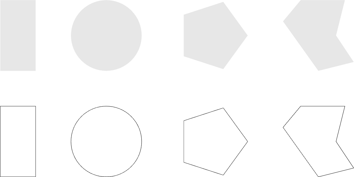
FIGURE 12 | Closed shapes and their surface equivalent

There is also the function surface which receives a curve or a list of curves and produces a surface limited by those curves. In fact:

• (surface-circle ... ) ≡ (surface (circle ... ))
• (surface-rectangle ... ) ≡ (surface (rectangle ... ))
• (surface-polygon ... ) ≡ (surface (polygon ... ))

In this tutorial you were introduced to Rosetta’s tools from drawing two-dimensional entities such as lines, curves, shapes and surfaces. These constitute the basic tools for creating any two-dimensional drawing so it is important that we know how to use them well. In the next tutorial we will move on to the third dimension and see what tools there are in Rosetta for creating and working with solid primitives. When you’re ready click the link below.