Data Preparation

Variable Encoding

Despite the heavy popularity of sklearn, unfortunatelly it does not deal with anything but numeric variables. For this reason, variable encoding has to be one of the first transformations to apply.

Ordinal Encoding

The easiest encoding is the ordinal one, but only shall be applied to binary and ordinal variables.

The usual way to do it is trough the use of the OrdinalEncoder and LabelEncoder, both from de sklearn.preprocessing package, however their usage is difficult to manage, in particular to impose the desired order.

A simple alternative is to use the replace from the DataFrame class, where the coding is explicitly made through the encoding dictionary.

from pandas import read_csv, DataFrame
from dslabs_functions import get_variable_types, encode_cyclic_variables, dummify

data: DataFrame = read_csv("data/stroke_mvi.csv", index_col="id", na_values="")
vars: dict[str, list] = get_variable_types(data)

yes_no: dict[str, int] = {"no": 0, "No": 0, "yes": 1, "Yes": 1}
residence_type_values: dict[str, int] = {"Rural": 0, "Urban": 1}

encoding: dict[str, dict[str, int]] = {
    "Residence_type": residence_type_values,
    "hypertension": yes_no,
    "heart_disease": yes_no,
    "ever_married": yes_no,
    "stroke": yes_no,
}
df: DataFrame = data.replace(encoding, inplace=False)
df.head()

	age	avg_glucose_level	bmi	gender	work_type	smoking_status	hypertension	heart_disease	ever_married	Residence_type	stroke
id
9046	67.0	228.69	36.600000	Male	Private	formerly smoked	0	1	1	1	1
51676	61.0	202.21	28.893237	Female	Self-employed	never smoked	0	0	1	0	1
31112	80.0	105.92	32.500000	Male	Private	never smoked	0	1	1	0	1
60182	49.0	171.23	34.400000	Female	Private	smokes	0	0	1	1	1
1665	79.0	174.12	24.000000	Female	Self-employed	never smoked	1	0	1	0	1

In the code above, we encoded all the binary variables, since the order among the values is irrelevant. Naturally, we could have chosen any order among the values, but in that case we would loose some information, which consequently would bias the training of models.

In order to choose the order to consider for each variable, we may start by collecting the individual values for each symbolic var.

for v in vars["symbolic"]:
    print(v, data[v].unique())

gender ['Male' 'Female' 'Other']
work_type ['Private' 'Self-employed' 'Govt_job' 'children' 'Never_worked']
smoking_status ['formerly smoked' 'never smoked' 'smokes']

Unexpectadly, the gender variable presents 3 different values, which makes it non-binary. We opt to code Female as 0, Male as 2, and Other as 1, considering it represents someone in between, meaning the value shouldn't be closer to any of the traditional values.

gender_values: dict[str, int] = {"Female": 0, "Other": 1, "Male": 2}
work_values: dict[str, int] = {
    "children": 0,
    "Never_worked": 1,
    "Self-employed": 2,
    "Private": 3,
    "Govt_job": 4,
}
status_values: dict[str, int] = {"never smoked": 0, "formerly smoked": 1, "smokes": 2}

encoding: dict[str, dict[str, int]] = {
    "gender": gender_values,
    "work_type": work_values,
    "smoking_status": status_values,
}

df: DataFrame = df.replace(encoding, inplace=False)
df.head()

	age	avg_glucose_level	bmi	gender	work_type	smoking_status	hypertension	heart_disease	ever_married	Residence_type	stroke
id
9046	67.0	228.69	36.600000	2	3	1	0	1	1	1	1
51676	61.0	202.21	28.893237	0	2	0	0	0	1	0	1
31112	80.0	105.92	32.500000	2	3	0	0	1	1	0	1
60182	49.0	171.23	34.400000	0	3	2	0	0	1	1	1
1665	79.0	174.12	24.000000	0	2	0	1	0	1	0	1

The logic for the rest of the variables shall be similar. Of course, if we have domain knowledge the choice of the order is natural, and there shouldn't be any doubt about it. Otherwise, we need to pick an order that seems to make sense in helping to descriminate among the class variables.

The smoking_status variable is an example of a situation where common sense is everything we need. Never having smoked (never smoked) aligns more closely with having quit smoking (formerly smoked) than actively smoking (smokes).

Cyclic variables

Among the ordinal variables there are some that instead of having a sequential order, show a cyclic one. Examples of these are season and day of the week.

In these cases, there is no right choice to use as the first or the last one, and so we need a different strategy to encode them.

The common methods applied nowadays to encode each one of these variables is to create two variables per each one, using trigonometric functions to simulate an angle. Say for a var variable we create two new variables to encode it - var_sin and var_cos.

In this manner, if var assumes a value x between 0 and x_max, then var_sin becomes x_sin and var_cos becomes x_cos given below.

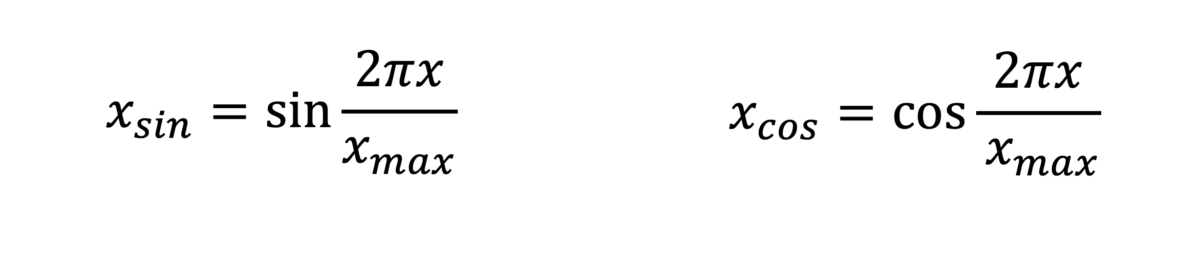
In order to do so, we just need to map the original values from 0 to x_max to values between 0 and (2pi * x / x_max).

from math import pi, sin, cos

data: DataFrame = read_csv(
    "data/algae.csv",
    index_col="date",
    na_values="",
    parse_dates=True,
    infer_datetime_format=True,
)

season_val: dict[str, float] = {
    "spring": 0,
    "summer": pi / 2,
    "autumn": pi,
    "winter": -pi / 2,
}
lov: dict[str, int] = {"low": 0, "medium": 1, "high": 2}
encoding: dict[str, dict] = {
    "river_depth": lov,
    "fluid_velocity": lov,
    "season": season_val,
}

data = data.replace(encoding)
data.head()

	pH	Oxygen	Chloride	Nitrates	Ammonium	Orthophosphate	Phosphate	Chlorophyll	fluid_velocity	river_depth	season
date
2018-09-30	8.10	11.4	40.02	5.33	346.67	125.67	187.06	15.6	1	0	3.141593
2018-10-05	8.06	9.0	55.35	10.42	233.70	58.22	97.58	10.5	1	0	3.141593
2018-10-07	8.05	10.6	59.07	4.99	205.67	44.67	77.43	6.9	2	0	3.141593
2018-10-09	7.55	11.5	4.70	1.32	14.75	4.25	98.25	1.1	2	0	3.141593
2018-10-11	7.75	10.3	32.92	2.94	42.00	16.00	40.00	7.6	2	0	3.141593

and then create the two new variables from the angle.

def encode_cyclic_variables(data: DataFrame, vars: list[str]) -> None:
    for v in vars:
        x_max: float | int = max(data[v])
        data[v + "_sin"] = data[v].apply(lambda x: round(sin(2 * pi * x / x_max), 3))
        data[v + "_cos"] = data[v].apply(lambda x: round(cos(2 * pi * x / x_max), 3))
    return


data: DataFrame | None = encode_cyclic_variables(data, ["season"])
if data is not None:
    data.head()

Dummification or One-hot Encoding

Dealing with nominal variables is another story. Indeed, by definition there is no order among the values assumed by the variable. When after exploring all possible perspectives, we are not able to specify an acceptable order among those variables the only solution is dummification.

This consists on creating a new variable for each possible value from the original one, removing it from the dataset.

Note, however, that a small number of values leads to the creation of several new variables, creating a much sparser dataset. And so, we shall avoid it as much as possible.

Additionaly, do not dummify the class variable, since it will transform a simple multi label classification problem into a multi class problem.

In order to apply dummification, we can make use of the OneHotEncoder from the package sklearn.preprocessing. The pandas.DataFrame.getDummies is much less interesting since it isn't able to apply the same encoder to different parts of a dataset, while the first one is.

For example, after dummifying the algae dataframe, we get a new one with 18 variables, instead of the 11 original ones, since each one of the three symbolic variables had three different values.

As we saw, we could have considered them as ordinal or cyclic and avoid the increasing of dimensionality.

from numpy import ndarray
from pandas import DataFrame, read_csv, concat
from sklearn.preprocessing import OneHotEncoder


def dummify(df: DataFrame, vars_to_dummify: list[str]) -> DataFrame:
    other_vars: list[str] = [c for c in df.columns if not c in vars_to_dummify]

    enc = OneHotEncoder(
        handle_unknown="ignore", sparse_output=False, dtype="bool", drop="if_binary"
    )
    trans: ndarray = enc.fit_transform(df[vars_to_dummify])

    new_vars: ndarray = enc.get_feature_names_out(vars_to_dummify)
    dummy = DataFrame(trans, columns=new_vars, index=df.index)

    final_df: DataFrame = concat([df[other_vars], dummy], axis=1)
    return final_df


data: DataFrame = read_csv(
    "data/algae.csv", index_col="date", na_values="", parse_dates=True, dayfirst=True
)
vars: list[str] = ["river_depth", "fluid_velocity", "season"]
df: DataFrame = dummify(data, vars)
df.head(5)

	pH	Oxygen	Chloride	Nitrates	Ammonium	Orthophosphate	Phosphate	Chlorophyll	river_depth_high	river_depth_low	river_depth_medium	fluid_velocity_high	fluid_velocity_low	fluid_velocity_medium	season_autumn	season_spring	season_summer	season_winter
date
2018-09-30	8.10	11.4	40.02	5.33	346.67	125.67	187.06	15.6	False	True	False	False	False	True	True	False	False	False
2018-10-05	8.06	9.0	55.35	10.42	233.70	58.22	97.58	10.5	False	True	False	False	False	True	True	False	False	False
2018-10-07	8.05	10.6	59.07	4.99	205.67	44.67	77.43	6.9	False	True	False	True	False	False	True	False	False	False
2018-10-09	7.55	11.5	4.70	1.32	14.75	4.25	98.25	1.1	False	True	False	True	False	False	True	False	False	False
2018-10-11	7.75	10.3	32.92	2.94	42.00	16.00	40.00	7.6	False	True	False	True	False	False	True	False	False	False