Programming for Architecture
1 Preface
This book was born in 2007, following an invitation to teach an introductory programming course to architecture students at Instituto Superior Técnico (IST). The original motivation for this course was the same as for several other courses: just like Mathematics and Physics, Programming has become one of the fundamental courses that constitute the basic education of any IST student.
With this premise, it did not seem to be a subject that would entice the student’s interest, particularly since it was not very clear the contribution it could have to the architectural curriculum. To contradict that first impression, I decided to include in the course’s syllabus some applications of Programming in Architecture. To that end, I had a conversation with several architectural students and teachers and asked them to explain to me what they did and how they did it. What I heard and saw was revealing.
Despite the enormous progresses that Computer-Aided-Design (CAD) and Building Information Modeling (BIM) brought to the profession, the truth is that its use continues to be manual, laborious, repetitive and boring. The creation of a digital model in a CAD or BIM tool requires extreme attention to detail, distracting the architect from what is fundamental: the idea. Frequently, the obstacles found end up forcing the architect to simplify the original idea. To make things worse, the obstacles do not end when the model is finally created. On the contrary, they become aggravated when inevitable design changes need to be made to that model.
In general, CAD and BIM tools are conceived to make the most common tasks easier, in detriment of other less common or sophisticated tasks. In fact, for an architect interested in modeling more complex shapes, the tools used can present several limitations. However, those limitations are only deceptions since they can be overcome with the aid of programming. Programming allows a CAD or BIM tool to be amplified with new capabilities, thus eliminating the obstacles that hinder the architect’s design process.
The programming practice is intellectually stimulating but it is also very challenging. Not only does it require mastering a new language, but it also implies a new way of thinking, an effort that, frequently, makes people give up. Nevertheless, those that prevail overcome the initial difficulties and acquire the skills to go further in the creation of innovative architectural solutions.
This book is meant for those architects.
2 Introduction
Throughout history, humanity has accumulated enormous amounts of knowledge. That knowledge is of extreme importance for our survival and, therefore, needs to be passed to the following generations. To this end, a series of mechanisms were invented. Firstly, oral transmission, from one person to a small group of people. Secondly, written transmission, consisting in documenting knowledge. This approach has the great advantage of reaching out to a much larger group of people and of significantly reducing the risk of knowledge loss. In fact, the written word allows us to preserve knowledge for long periods of time, safe from the inevitable corruption that occurs on a long chain of oral transmissions.
It is thanks to the written word that mankind can understand vast amounts of knowledge, some of which date back thousands of years. Unfortunately, the written word has not always been able to accurately transmit what the author had in mind. The natural language is ambiguous and it evolves with time, making the interpretation of written texts a subjective task: there are omissions, imprecisions, errors, and ambiguities, both when we write a text and when we read it, which can turn knowledge transmission into a fallible endeavor.
When rigor is needed in the transmission of knowledge, relying on the receptor’s abilities to understand it can have disastrous outcomes. In fact, throughout history we can find many catastrophic events caused solely by insufficient or incorrect transmission of knowledge. To avoid these problems, more accurate languages were invented. Mathematics, in particular, has obsessively been seeking to construct a language of absolute rigor over the past millennia. This allows for a much more accurate transmission of knowledge than in other areas, but it still requires a human to understand it.
To better understand this problem, let us consider one concrete example: the calculus of the factorial of a number. If we assume that the person to whom we want to transmit that knowledge knows beforehand the meaning of numbers and arithmetic operations, we could tell him that, to calculate the factorial of a number, one must multiply every number from one until that number. Unfortunately, that description is inaccurate, because it does not state that only integer numbers are to be multiplied. To avoid these imprecisions and simultaneously make the information more compact, Mathematics developed a set of symbols and concepts that should be understood by everyone. For example, to define the integer sequence of numbers between \(1\) and \(9\), Mathematics allows us to write \(1,2,3,\ldots,9\). In the same manner, instead of referring to a number, Mathematics invented the concept of variable: a name that refers to some “thing” that can be used in several parts of a mathematical statement, always representing the same “thing”. In this way, Mathematics allows us to more accurately express the factorial computation as follows:
\[n! = 1\times 2\times 3\times \cdots{} \times n\]
But is this definition rigorous enough? Is it possible to interpret it without guessing the author’s intention? For a human being, maybe. However, if we want to be as rigorous as possible, then we must admit that there is one detail in this definition that requires some imagination: the ellipsis. The ellipsis indicates that the reader must imagine what should be in its place. Although most readers will correctly understand that the author meant the multiplication of the subsequent numbers, some might think to replace the ellipsis with something else.
Even if we exclude this last group of people from our target audience, there are still other problems with the previous definition. Let us imagine, for example, the factorial of \(2\). What will be its value? If we use \[n = 2\] in the formula, we get:
\[2! = 1\times 2\times 3\times \cdots{} \times 2\]
In this case, the computation makes no sense, which shows that, in fact, imagination is needed for more than just understanding the ellipsis: the number of terms to consider depends on the number to which we want to calculate the factorial.
Assuming that our reader has enough imagination to figure out this particular detail, he would easily calculate that \(2!=1\times 2=2\). But even so, there will be cases where it is not that clear. For example, what is the factorial of zero? The answer does not appear to be obvious. What about the factorial of \(-1\)? Again, it is not clear. And the factorial of \(4.5\)? Once again the formula says nothing regarding these situations and our imagination cannot guess the correct procedure.
Would it be possible to find a way of transmitting the knowledge required to compute the factorial function that minimizes imprecisions, gaps, and ambiguities? Let us try the following variation of the factorial function definition:
\[n!= \begin{cases} 1, & \text{if $n=0$}\\ n \cdot (n-1)!, & \text{if $n\in \mathbb{N}$.} \end{cases}\]
Have we reached the necessary rigor that dispenses imagination on the reader’s part? One way to find out is to reanalyze the cases that had previously caused problems. First of all, there is no ellipsis, which is positive. Secondly, for the factorial of the number \(2\), we have:
\[2!=2\times 1!=2\times (1\times 0!)=2\times (1\times 1)=2\times 1=2\]
which means that there is no ambiguity. Finally, we can see that it makes no sense trying to determine the factorial value of \(-1\) or \(4.5\) because this function can only be applied to \(\mathbb{N}_0\) members.
This example shows that, even in Mathematics, there are different levels of rigor in the different ways of expressing knowledge. Some require more imagination than others but, in general, they have been enough for mankind to preserve knowledge throughout history.
This state of affairs changed in the last decades: mankind has now a partner which has been giving an enormous contribution to its progress: the computer. This machine has the extraordinary capability of being instructed on how to execute a complex set of tasks. Programming is essentially all about transmitting to a computer the knowledge needed to solve a specific problem. This knowledge is called a program. Because they are programmable, computers have been used for the most diversified ends and they have radically changed the way we work. Unfortunately, the computer’s extraordinary ability to learn comes with an equally extraordinary lack of imagination. A computer does not assume or imagine, it just rigorously interprets the knowledge transmitted in the form of a program.
Since it has no imagination, the computer depends critically on the way we present it the knowledge that we wish to transmit, which must be described in a language that allows for no ambiguity, gaps, or imprecision. A language with these characteristics is generally called a programming language.
2.1 Programming Languages
For a computer to be able to solve a problem it is necessary to describe the process of solving the problem in a language that it understands. Unfortunately, the language that a computer “innately” understands is extremely poor, making the description of how to solve a non-trivial problem a very exhausting, tedious and complex task. The countless programming languages that have been invented aim at alleviating the programmer’s burden, by introducing linguistic elements capable of simplifying those descriptions. For example, the concepts of function, sum, matrix or rational number do not exist natively in computers but many programming languages allow their usage in order to simplify the description of scientific calculus. Naturally, this implies a process that transforms the programmer’s descriptions into instructions that computers can understand. This process is called compilation and although it is relatively complex, we only need to know that it allows us to use programming languages that are closer to the thinking capabilities of humans, than those of computers.
Compilation is of extreme importance because it allows us to use programming languages not only to instruct a computer on how to solve a problem, but also to explain that process accurately to another human being. In this way, much like Mathematics, programming languages become a way of transmitting knowledge and, in fact, they are even more rigorous than Mathematics.
There is a great diversity of programming languages, some better equipped than others to solve specific problems. This means that choosing a programming language should depend on the kind of problems we wish to solve, but it should not be a full commitment. For a programmer, it is much more important to understand the fundamentals and techniques of programming than to master one language or another. However, to better understand these fundamentals, it is convenient to exemplify them in a concrete programming language.
As this document will focus on programming for architecture, we will use a programming language that is geared towards solving geometrical problems. There are many languages that serve this purpose, most commonly associated with Computer Aided Design (CAD) or Building Information Modeling (BIM). ArchiCAD, for instance, offers a programming language called GDL, an acronym for Geometric Description Language that enables users to program multiple geometric forms. In the case of AutoCAD, the language used is called AutoLisp, a dialect of a famous programming language called Lisp. A third option is the RhinoScript language, available for Rhinoceros 3D. Despite these languages seeming very different from each other, the concepts behind them are very similar. These fundamental concepts of programming will be the main focus of our study. However, for pedagogical reasons, it is convenient to address them in a single language.
Unfortunately, GDL, AutoLisp, and RhinoScript were developed many years ago and they have not been updated, possessing many archaic characteristics that make them harder to learn and use. In order to ease the learning process while allowing our programs to run in different CAD environments, we are going to use a new language called Julia, which was purposely adapted for programming in architecture. Julia is freely available at https://julialang.org/. In this text we will explain the fundamentals of programming using Julia, not just because it is easier to learn, but also for its practical applicability. However, once learned, the reader should be able to apply these fundamentals to any other programming language.
In order to facilitate the programmer’s task, Julia can be used from a programming environment called Atom, which offers a text editor adapted to edit Julia’s programs, as well as a set of additional tools for error detection and debugging. This programming environment is shared with a freeware license and it is available at https://atom.io/.
2.1.1 Exercises 1
2.1.1.1 Question 1
Exponentiation \(b^n\)is an operation between two numbers \(b\) and \(n\). When \(n\) is a positive integer, exponentiation is defined as:
\[b^n = \underbrace{b \times b \times \cdots \times b}_n\]
To a reader not familiarized with exponentiation, the previous definition raises several questions that may not be evident: how many multiplications should actually be done? \(n\)?, \(n-1\)? What if \(n=1\)? Or \(n=0\)? Propose a definition for the exponentiation function that raises none of these questions.
2.1.1.2 Question 2
What is a program and what purpose does it serve?
2.1.1.3 Question 3
What is a programming language and what purpose does it serve?
2.2 The Julia Language
In this section we will learn about Julia programming language, which we will use throughout this text. But first, we are going to examine some aspects that are common to other languages.
2.2.1 Syntax, Semantics and Pragmatics
Every language has syntax, semantics, and pragmatics.
In simple terms, syntax is a set of rules that dictate the kind of sentence that can be written in a language. Without it, any concatenation of words could be a sentence. For example, given the words “John”, “cake”, “ate”, and “the”, the syntax rules of the English language tell us that - “John ate the cake” is a correct sentence, and that - “the ate cake John” is not. It is also important to note that, according to the English syntax, “The cake ate John” is also syntactically correct. This means that syntax is not enough to completely specify the rules of a language. In fact, syntax dictates how a sentence is constructed but says nothing in regards to its meaning. That is the job of semantics, which attributes meaning to a sentence, thus telling us that “The cake ate John” makes no sense. Finally, pragmatics sets the way sentences are commonly expressed. In a language, pragmatic changes depending on the context: the way two close friends talk with each other is different from the way two strangers talk.
These three aspects of a language are also present when we discuss programming languages. Unlike the natural languages we use to communicate between us, programming languages are characterized as being formal, obeying a set of simple and restrictive rules that can be mechanically processed.
In this document we will describe Julia’s syntax and semantics and, although there are mathematical formalisms to describe rigorously those two aspects, they require a mathematical sophistication that, given the nature of this work, is inappropriate. Hence, we will only use informal descriptions. Afterwards, as we introduce language elements, we will discuss the language pragmatics.
2.2.2 Syntax and Semantics of Julia
Compared to other programming languages, Julia’s syntax is simple and is based on the concept of expression.
An expression in Julia can be formed using primitive elements, such as numbers, or by the combination of those elements using an operation, such as the sum of two numbers. This simple definition allows us to build expressions of arbitrary complexity. However, it is important to remember that syntax restricts what can be written: the fact that we can combine expressions to create more complex ones does not mean we can write any combination of expressions. These combinations are restricted by syntactic rules, which we will describe throughout this text.
Much like syntax, Julia’s semantics is also simple when compared to other programming languages. As we will see, semantics is determined by the operators that are used in our expressions. For instance, the sum operator is used to add two numbers. An expression that combines this operator with, for example, the numbers \(3\) and \(4\) will have as meaning the sum between \(3\) and \(4\), i.e., \(7\). In a programming language, the semantics of an expression is given by the computer when it evaluates the expression.
2.2.3 The Evaluator
Every expression in Julia has a value. This concept is so important that Julia provides an evaluator, i.e., a program designed to evaluate expressions.
In Julia, the evaluator is shown as soon as we start working with the language. Once Julia is running, the user is presented with the text julia> (called prompt), meaning that Julia is waiting for the user to input an expression. Julia interacts with the user by executing a cycle that reads an expression, determines its value, and writes it. This cycle is traditionally called read-eval-print loop (abbreviated to REPL).
During the read phase, Julia reads an expression. In the evaluation phase, that expression is analyzed in order to produce a value. This analysis uses rules that dictate, for each case, the expression value. Finally, in the print phase, this value is printed so that the user can see it.
The existence of the read-eval-print loop makes Julia an interactive language that allows programs to be quickly developed by writing, testing, and correcting small fragments at a time.
2.3 Language Elements
In every programming language we have two important concepts: data and procedures. Data comprise the entities that we wish to manipulate. Procedures describe how to manipulate those entities.
In Mathematics, we can look at numbers as the data and at algebraic operations as the procedures. These operations allow us to combine numbers. For example, \(2\times 2\) is a combination. Another combination involving more data is \(2\times 2\times 2\), and using even more data \(2\times 2\times 2\times 2\). However, unless we want to spend time solving problems of elementary arithmetic, we should consider more elaborate operations that represent combination patterns. In the previous sequence of combinations, it is clear that the pattern emerging is the concept of exponentiation, which has been defined in Mathematics a long time ago. Exponentiation is therefore an abstraction of a succession of multiplications.
As in Mathematics, a programming language should contain data and procedures, should be capable of combining data and procedures to create more complex data and procedures, and should be able to abstract patterns, allowing the definition of new operations that represent those patterns.
Further ahead we will see how to define these abstractions in Julia. For now, let us take a closer look at the primitive elements of the language, i.e., the simplest entities that the language deals with.
2.3.1 Numbers
Numbers are one of the most primitive elements of Julia. Julia provides integers, fractions, reals, and other kinds of numbers. The syntax of the language includes different ways for the user to write those different kinds of numbers. Regarding semantics, numbers are very simple to evaluate: the value of a number is the number itself. For example, the value of 1 is 1.
In Julia, numbers can be exact or inexact. Exact numbers include integers, fractions and complex numbers with integer parts. Inexact numbers are all others, typically written in decimal or scientific notation, such as \(123.45\) or \(1.2345e2\).
2.4 Combinations
A combination is an expression that describes the application of an operator to its operands. For example, numbers can be combined using operations like the sum or product, e.g. \(1 + 2\) and \(1 + 2 \times 3\). The sum and product of numbers are two of the most primitive procedures provided by Julia. Naturally, many other operations can be used, including mathematical functions such as sine (\(\sin\)) or cosine (\(\cos\)). The syntax for functions, however, is slightly different: unlike arithmetic operators, like sum and product that use infix syntax, i.e., the operator appears between the operands, functions use prefix syntax, i.e., they appear before the operands, as in \(\sin 2\). Finally, there are also operators, such as factorial (abbreviated \(!\)) that are used with postfix syntax, as in \(5 !\).
In Julia, a combination can be created using a syntax similar to the one used in Mathematics, although with some small differences: functions are written in prefix syntax but function arguments are grouped with parentheses, as in sin(2). Arithmetic operators can also be treated as functions, as in +(1,2) but they are usually written using infix syntax, as in 1+2. In Julia, an expression is a primitive element or a combination of expressions with an operation. The expression 1+2 is a combination of the two primitive elements 1 and 2 through the primitive procedure +. In the case of 1+2*3, the combination is between the number 1 and the combination 2*3 because Julia follows the same precedence rules used in Mathematics. Therefore, the expression 1+2*3 is interpreted as 1+(2*3).
2.4.1 Exercises 2
2.4.1.1 Question 4
Explain the acronym REPL.
2.4.2 Evaluating Combinations
The evaluator determines a combination’s value by applying the procedure specified by the operator to the value of the operands. The value of an operand is designated as the argument of the procedure. The value of the combination 1+2*3 is the result of adding the value of 1 to the value of 2*3. As we have already seen, the value of 1 is \(1\) and 2*3 is a combination whose value is the result of multiplying 2 by 3, which is \(6\). Finally, by summing \(1\) with \(6\) we get \(7\).
> 2*3
6
> 1+2*3
7
2.4.3 Strings
Chains of characters (also called Strings) are another type of primitive data. A character is a letter, a digit or any kind of graphic symbol, including non-visible graphic symbols like blank spaces, tabs and others. A string is specified by a character sequence between quotations marks. Just like with numbers, the value of a string is the string itself:
> "Hi"
"Hi"
> "I am my own value"
"I am my own value"
Since a string is delimited by quotation marks, how can we create a string that contains quotation marks? For this and other special characters, there is one particular character that Julia interprets differently: when the character \ appears in a string, it tells Julia that the next characters must be evaluated in a special way. For example, to create the following string:
John said "Good morning!" to Peter.
We must write:
"John said \"Good morning!\" to Peter."
The character \ is called an escape character and allows the inclusion of characters in strings that would otherwise be difficult to input. This table shows examples of other special characters that need to be escaped.
Some valid escape characters in Julia.
As it happens with numbers, there are countless operators to manipulate strings. For example, to concatenate multiple strings we can use the * operator. The concatenation of several strings produces a single string with all the characters of those strings, in the same order:
> "1"*"2"
"12"
> "one"*"two"*"three"*"four"
"onetwothreefour"
> "I"*" "*"am"*" "*"a"*" "*"string"
"I am a string"
> "And I"*" am "*"another"
"And I am another"
To know how many characters there are in a string we have the length operator:
> length("I am string")
11
> length("")
0
Note that quotation marks define strings’ boundaries and are not considered characters. Besides strings and numbers, Julia has other kinds of primitive elements that will be addressed later.
2.5 Defining Functions
Mathematics offers a large set of operations that are defined based on the most basic ones. For example, the square of a number is an operation (also designated as a function) that, given a number, multiplies that number by itself. This function has the following mathematical definition:
\[x^2 = x \cdot x\]
Like in Mathematics, it is possible to define the square function in a programming language. In Julia, to obtain the square of the number 5, we write the combination 5*5. In general, given a number x, we square it by writing x*x. All that is left to do is associate a name indicating that, given a number x, we obtain its square by evaluating x*x. This is done in Julia as follows:
square(x) = x*x
As you can see from the square function definition, in order to define a function in Julia, we need to use the following syntax:
name (parameter1, ..., parametern) = body |
The function’s parameters are called formal parameters, and they are used in the body of the function to refer to the corresponding arguments. When we write square(5) in the evaluator, the number 5 is the argument of the function. During the calculation this argument is associated with the parameter x. The arguments of a function are also called actual parameters.
The definition of the square function declares that, in order to determine the square of a number x, we should multiply that number by itself (x*x). This definition associates the word square with a procedure, i.e., a description on how to obtain the desired result. Note that this procedure has parameters allowing its use with different arguments. As an example, we will evaluate the following expressions:
> square(5)
25
> square(6)
36
The previously explained rule to evaluate combinations is also valid for combinations that invoke user-defined functions. The evaluation of the expression square(1+2) first evaluates the 1+2 argument. The resulting value, \(3\), will then replace parameter x in the function. This means that the function’s body is evaluated with all occurrences of x replaced by the value 3 and, therefore, the final value will be the value of the combination 3*3, i.e., 9.
Formally, in order to invoke a function, one must construct a combination in which the first element is an expression whose value is the function we want to invoke, and the remaining elements are expressions whose values are the arguments that the function is supposed to use. The result of the combination’s evaluation is the value calculated by the function for those arguments.
The process of evaluating a combination follows three essential steps:
All elements in a combination are evaluated. The value of the first element must be a function.
The formal parameters are associated to the function’s arguments, i.e., the value of the remaining elements of that combination. Each parameter is associated to an argument, according to the order of parameters and arguments. An error occurs when the number of parameters does not match the number of arguments.
The function’s body is evaluated while considering the associations between parameters and arguments.
To better understand this process, it is useful to break it down to its most elementary steps. The following example shows the process of evaluating the expression \(((1+2)^2)^2\) step by step:
square(square(1+2))\(\downarrow\)square(square(3))\(\downarrow\)square(3*3)\(\downarrow\)square(9)\(\downarrow\)9*9\(\downarrow\)81
Julia does not distinguish between predefined functions and functions created by the user. This means that, just like predefined functions, user-defined functions can be used to create new functions. For example, after defining the square function, we can define the function that calculates the area of a circle with radius \(r\), using the formula \(\pi * r^2\):
circle_area(radius) = pi*square(radius)
Naturally, during the evaluation of the expression that computes the area of a circle, the square function is invoked. This is visible in the following evaluation sequence:
circle_area(2)\(\downarrow\)pi*square(2)\(\downarrow\)3.14159*square(2)\(\downarrow\)3.14159*2*2\(\downarrow\)3.14159*4\(\downarrow\)12.5664
Defining a function causes an association between a procedure and a name. In order to retrieve this association whenever the function is being used, Julia needs to store the association in the computer’s memory. The memory that contains these associations is called the evaluation environment.
Note that this environment exists only while we are using the program. When the program is shut down, that environment is lost. In order to avoid losing those definitions, they should be saved in a file. This means that, despite the usefulness of the REPL for testing the definitions, these should be written in files to preserve them for future use. Fortunately, programming environments, such as Atom, facilitate this workflow.
2.5.1 Exercises 3
2.5.1.1 Question 5
Define the function double, which calculates the double of a given number.
2.6 Names
Defining a function involves assigning names, not only for the function itself, but also for its parameters.
In Julia, there are a few restrictions regarding names: they must begin with a letter, the underscore character, or a Unicode symbol (in practice, only a subset of Unicode is allowed). The remaining characters can also include !, digits and many more Unicode symbols. However, note that it is not possible to use names that are already reserved by the language. We will see some of them soon.
Pragmatically speaking, the creation of names should take some rules into consideration:
Avoid using digits, if possible.
For portability reasons, accented characters should be avoided.
If a name has more than one word, those words should be concatenated or, when the result is difficult to understand, the names should be separated by an underscore (_). For example, a function that computes the area of a circle might be named circle_area.
The choice of names will have a significant impact on the program’s legibility. Let us consider for example the area \(A\) of a triangle with base \(b\) and height \(c\), which can be defined mathematically by:
\[A(b,c) = \frac{b \cdot c}{2}\]
In Julia we will have:
A(b, c) = (b*c)/2
Note that the Julia definition is identical to the corresponding mathematical expression. However, if we did not know beforehand what the purpose of this function was, we would hardly understand it just by looking at its name and/or at the names of the parameters. Therefore, and contrary to Mathematics, the names that we assign in Julia should have a clear meaning. Instead of writing "A", it is preferable that we write "triangle-area" and, instead of writing "b" and "c", we should write "base" and "height", respectively. Taking these aspects into consideration, we can present a more meaningful definition:
triangle_area(base, height) = (base*height)/2
As the number of definitions grow, names become particularly important for the reader to quickly understand the written program, so it is crucial that names are carefully chosen.
2.6.1 Exercises 4
2.6.1.1 Question 6
Function that calculates the volume of a sphere;
Function that tests if a number is a prime number;
Function that converts a measurement in centimeters into inches.
2.6.1.2 Question 7
Define the function radians_from_degrees that receives an angle in degrees and computes the corresponding value in radians. Note that \(180\) degrees are \(pi\) radians.
2.6.1.3 Question 8
Define the function degrees_from_radians that receives an angle in radians and computes the corresponding value in degrees.
2.6.1.4 Question 9
Define a function that calculates the perimeter of a circle given its radius.
2.6.1.5 Question 10
Define a function that calculates the volume of a parallelepiped from its length, width and height.
2.6.1.6 Question 11
Define a function that calculates the volume of a cylinder from its height and base radius. The volume corresponds to multiplying the area of the base by the cylinder’s height.
2.6.1.7 Question 12
Define a function average that calculates the average value between two numbers. For example: average(2, 3) \(\rightarrow\) 2.5.
2.7 Predefined Functions
The possibility of defining new functions is fundamental for increasing the language’s flexibility and its ability to adapt to the problems we want to solve. The new functions, however, must be defined in terms of others that were either defined by the user or, at most, predefined in the language.
As we will see, Julia has a vast set of predefined functions. In many cases, they suffice for what we want to do. Nevertheless, we should not restrain from defining new functions whenever we deem it necessary.
The name sqrt is a contraction of the words square and root
Some mathematical functions predefined in Julia.
Function
Arguments
Result
abs
A number
The absolute value of the argument.
sin
A number
The sine of the argument (in radians).
cos
A number
The cosine of the argument (in radians).
atan
One or two numbers
With only one argument, the arc tangent of the argument (in radians). With two arguments, the arc tangent of the division between the first and the second, where the sign of the arguments is used to determine the quadrant.
sqrt
A number
The square root of the argument.
exp
A number
The exponential value with base \(e\) of the argument.
^
Two numbers
The first argument raised to the power of the second argument.
log
One or two arguments
With one argument, the natural logarithm of the argument. With two arguments, the logarithm of the second argument with the first argument as its base.
max
Multiple Numbers
The highest argument.
min
Multiple Numbers
The lowest argument.
round
A number
Rounds the argument to the nearest integer.
floor
A number
Rounds down the argument to the nearest integer.
ceil
A number
Rounds up the argument to the nearest integer.
Julia’s predefined math functions.
2.7.1 Exercises 5
2.7.1.1 Question 13
\(\sqrt{\frac{1}{\log 2^{\left|(3-9\log 25)\right|}}}\)
\(\frac{\cos^4 \frac{2}{\sqrt 5}}{\arctan 3}\)
\(\frac{1}{2} + \sqrt 3 + \sin^{\frac{5}{2}} 2\)
2.7.1.2 Question 14
log(sin(2^4+floor(atan(pi))/sqrt(5)+pi))
cos(cos(cos(0.5)))^5
sin(cos(sin(pi/3)/3)/3)
2.7.1.3 Question 15
Define the function odd that, for a given number, evaluates if it is odd, i.e., if the remainder of that number when divided by two is one.
2.7.1.4 Question 16
The area \(A\) of a pentagon inscribed in a circle of radius \(r\) is given by the following expression: \[A = \frac{5}{8}r^2\sqrt{10 + 2\sqrt{5}}\] Define a function that calculates this area and test it with values of your choice.
2.7.1.5 Question 17
Define a function that calculates the volume of an ellipsoid with semi-axes \(a\), \(b\) and \(c\). This volume can be obtained by using the formula: \(V=\frac{4}{3}\pi a b c\)
2.8 Arithmetic in Julia
Julia is capable of dealing with several types of numbers, from integers to complex numbers, as well as fractions. Some of those numbers, like \(\sqrt 2\) or \(pi\), do not have a rigorous representation based in numerals and, for that reason, Julia classifies them as inexact numbers to emphasize the fact that we are dealing with an approximate value. When an inexact number is used in an arithmetic operation, the result will also be inexact, so the inexactness is said to be contagious.
Finitude is another feature of some types of numbers, meaning that those numbers cannot surpass a certain limit, above which every number is represented by infinity, as you can see by the following example that uses inexact numbers:
> 10.0^10
1.0e10
> 10.0^100
1.0e100
> 10.0^1000
Inf
Note that Inf (or -Inf) is Julia’s way of saying that a number exceeds the representation capacity. The number is not infinite, as one might think, but merely a value excessively big.
There is also another problem regarding inexact numbers: round-off errors. As an example, consider the obvious equality \((4/3-1)*3-1=0\) and note its result in Julia:
> (4/3-1)*3-1
-2.220446049250313e-16
As is possible to see, we did not obtain the correct result due to representation and round-off errors: 4/3 cannot be represented with a finite number of digits. This round-off error is then propagated to the remaining operations, producing a value that is not zero but is close to zero.
2.8.1 Exercises 6
2.8.1.1 Question 18
Translate the following definition to Julia: \[f(x)=x-0.1\cdot{}(10\cdot{}x-10)\]
2.8.1.2 Question 19
In mathematical terms, whatever the argument used in the previously mentioned function is, the result should always be \(1\), since \[f(x)=x-0.1\cdot{}(10\cdot{}x-10)=x-(x-1)=1\] Using the function defined in the previous exercise, evaluate the following expressions and explain the results:
f(5.1)
f(51367.7)
f(176498634.7)
f(1209983553611.9)
f(19843566622234755.9)
f(553774558711019983333.9)
2.8.1.3 Question 20
We wish to create a flight of stairs with \(n\) treads, covering a height \(a\) in meters. Considering that each step has a rise height \(h\) and a tread depth \(d\) that obey to the following proportion: \[2h+d=0.64\]
Define a function that, from a given height to cover and the number of treads, computes the length of the flight of stairs.
2.9 Name Evaluation
The primitive elements presented so far, such as numbers and strings, evaluate to themselves, i.e., the value of an expression composed only by a primitive element is the primitive element itself. For names, this is no longer true.
Names have a special meaning in Julia. Note that when we define a function, we give it a name. Its formal parameters are names as well. When a combination is written, the evaluator uses the function definition associated with the name of the operator of the combination. This means that the value of the operator in a combination is the associated function. If we had defined the function square, as suggested in section Defining Functions, we could verify this behavior by testing the following expressions:
> square(3)
9
> square
square (generic function with 1 method)
As we can see, the value of the name square is an entity that Julia describes using a special notation. This entity is, as shown, a function. The same behavior happens with any other function:
> +
+ (generic function with 178 methods)
> *
* (generic function with 377 methods)
As we have seen, the sum + and multiplication * signs are some of the predefined names of the language. For example, the symbol pi is also predefined and associated with an approximated value of \(\pi\):
> pi
π = 3.1415926535897...
However, when the body of the expression is evaluated, the value of a name assigned to a parameter of the function is the corresponding argument during the function call. For example, in the combination square(3), after figuring out that the value of square is a function and that the value of 3 is \(3\), the evaluator then evaluates the body of the function, replacing the name x, whenever necessary, with the same \(3\) that was previously assigned to the function’s parameter x.
2.10 Conditional Expressions
There are many operations in which the result is dependent on a specific test. For example, the mathematical function \(|x|\), which computes the absolute value of \(x\), is equivalent to the symmetric of \(x\) if \(x\) is negative, and to \(x\) itself otherwise. Using the mathematical notation we have:
\[|x|= \begin{cases} -x, & \text{if $x<0$}\\ x, & \text{otherwise.} \end{cases}\]
This function needs to test if the argument is negative in order to choose one of two alternatives: it either evaluates for the number itself or for its symmetrical value.
Expressions whose result depends on one or more tests are called conditional expressions.
2.10.1 Logical Expressions
A conditional expression follows the structure “if expression then ..., otherwise ...”. The expression that determines whether to use the branch “if” or the branch “otherwise”, is called a logical expression and is characterized for having its value interpreted as either true or false. For example, the logical expression x < 0 tests if the value of x is less than zero; if it is, the expression’s evaluation will return true, otherwise it will return false.
2.10.2 Logical Values
Boolean algebra was named after George Boole, the English mathematician that invented the algebra of logic.
2.11 Predicates
In the most usual case, a logical expression is the application of a function to a set of arguments. In this case, the function is known as a predicate: a function that produces only true or false.
2.11.1 Arithmetic Predicates
The mathematical relational operators \(<\),\(>\),\(=\),\(\leq\) and \(\geq\) are some of the most simple predicates. These operators compare numbers. Their use in Julia follows infix notation and are written respectively <,>,==, <= and >=. Some examples are:
> 4 > 3
true
> 4 < 3
false
> 2+3 <= 6-1
true
> 2+3 == 6-1
true
Note that arithmetic equality in Julia uses ==. This is to avoid any confusion with function definitions, which use =.
2.12 Predicates with a Variable Number of Arguments
An important property of the arithmetic predicates <,>,==, <= and >= is that they accept any number of arguments. Whenever there is more than one argument, the predicate is applied sequentially to pairs of arguments. This property can be seen in the following examples:
> 1 < 2 < 3
true
> 1 < 2 < 2
false
2.13 Recognizers
Apart from relational operators, there are many other predicates in Julia, like iszero, which tests if a number is zero:
> iszero(1)
false
> iszero(0)
true
Note that the operator iszero is used to recognize a particular element (zero) in a data type (numbers). These types of predicates are known as recognizers.
2.14 Logical Operators
In order to combine logical expressions together, we have the conjunction &&, the disjunction ||, and the negation ! operators. While the conjunction and the disjunction operators take two arguments and are written in infix notation, the negation operator takes just one argument in prefix notation. The value of such combinations is determined by the following rules:
&& evaluates arguments from left to right until one of them is false, in which case it returns false. If none of the arguments are false, the && operator returns true.
|| evaluates arguments from left to right until one of them is true, in which case it returns true. If none of the arguments are true, the || operator returns false.
! evaluates to true if the argument is false, and evaluates to false if the argument is true.
2.14.1 Exercises 7
2.14.1.1 Question 21
(2 > 3 || !(2 == 3)) && 2 < 3
!(1 == 2 || 2 == 3)
1 < 2 || 1 == 2 || 1 > 2
2.14.2 Exercises 8
2.14.2.1 Question 22
What is a conditional expression? What is a logical expression?
2.14.2.2 Question 23
What is a logical value? Which logic values does Julia provide?
2.14.2.3 Question 24
What is a predicate? Give examples of predicates used in Julia.
2.14.2.4 Question 25
What is a relational operator? Give examples of relational operators used in Julia.
2.14.2.5 Question 26
What is a logical operator? Give examples of logical operators used in Julia.
2.14.2.6 Question 27
What is a recognizer? Give examples of recognizers in Julia.
2.14.2.7 Question 28
\(x<y\)
\(x\leq y\)
\(x<y\wedge y<z\)
\(x<y\wedge x<z\)
\(x\leq y \leq z\)
\(x\leq y < z\)
\(x< y \leq z\)
2.15 Selection
If we look at the mathematical definition of the absolute value function:
\[|x|= \begin{cases} -x, & \text{if $x<0$}\\ x, & \text{otherwise} \end{cases}\]
we notice that it uses a conditional expression in the form of
\[\begin{cases} \mathit{consequent}, & \text{if} \quad\mathit{condition}\\ \mathit{alternative}, & \text{otherwise} \end{cases}\]
that translates to common language as “if condition then consequent, otherwise alternative”.
The evaluation of a conditional expression is done through the evaluation of the condition. If the condition is true, the consequent is evaluated, and if it is false the alternative is evaluated.
Just like Mathematics, Julia supports conditional expressions. To that end, it provides two different forms. We will start with the simplest one, called the ternary operator, whose syntax is the following:
condition ? consequent : alternative |
The value of a conditional expression is computed in the following way:
The condition is evaluated;
If the previous evaluation is true, the value of the conditional expression is the value of the consequent;
Otherwise (i.e., if the condition turns out to be false), the value of the conditional expression is the value of the alternative.
This behavior can be verified by the following examples:
> 3 > 2 ? 1 : 2
1
> 3 > 4 ? 1 : 2
2
Using a conditional expression, we can now define the absolute value function by translating its mathematical definition to Julia:
abs(x) = x < 0 ? -x : x
The purpose of the conditional expression is to define functions whose behavior depends on one or more conditions. For example, consider the max function that takes two numbers as arguments and returns the largest. To define such a function we only need to test if the first number is bigger than the second. If it is, the function returns the first argument, otherwise it returns the second one. Based on this logic, we can write:
max(x, y) = x > y ? x : y
The other form of Julia’s conditional expressions uses the words if, else and end, according to the following syntax:
if condition consequent else alternative end |
Therefore, the max function can be alternatively written as:
max(x, y) =
if x > y
x
else
y
end
Another far more interesting example is the mathematical function \(\operatorname{sgn}\), also known as signum (Latin for “sign”). This function could be interpreted as the dual function of the absolute value function, since \(x=\operatorname{sgn}(x) |x|\). The sgn function is defined as:
\[\operatorname{sgn} x = \begin{cases} -1 & \text{if $x<0$} \\ 0 & \text{if $x = 0$} \\ 1 & \text{otherwise}\end{cases}\]
In natural language, we would say that if \(x\) is negative, the \(\operatorname{sgn} x\) value is \(-1\), otherwise, if \(x\) is \(0\), the value is \(0\), otherwise the value is \(1\). This shows that the above expression uses two conditional expressions stacked in the following way:
\[\operatorname{sgn} x = \begin{cases} -1 & \text{if $x<0$} \\ \begin{cases} 0 & \text{if $x = 0$} \\ 1 & \text{otherwise}\end{cases} & \text{otherwise}\end{cases}\]
To define this function in Julia, two conditional expressions must be used:
sgn(x) = x < 0 ? -1 : (x == 0 ? 0 : 1)
2.15.1 Multiple Selection
When we begin stacking multiple conditional expressions, the program becomes increasingly harder to read. In this case, there is an alternative syntax that might make the function’s definition easier to read. The syntax is as follows:
if condition1 |
consequent1 |
elseif condition2 |
consequent2 |
... |
elseif conditionn |
consequentn |
else |
alternative |
end |
The previous form takes as many pairs conditioni–consequenti as needed. Each of these pairs is called a clause. The semantics of a multiple conditional expression is based on the sequential evaluation of the "condition" in each clause until one of them returns true. In that case, the corresponding "consequent" expression is evaluated and the resulting value is returned. If none of the conditions are true, the value of the alternative is returned.
Using the if form makes the sgn function slightly easier to understand:
sgn(x) =
if x < 0
-1
elseif x == 0
0
else
1
end
2.15.2 Exercises 9
2.15.2.1 Question 29
Define the function sum_largest that, given three numbers as arguments, calculates the sum of the two highest values.
2.15.2.2 Question 30
Define the function max3 that, given three numbers as arguments, returns the maximum value.
2.15.2.3 Question 31
Define the function second_largest that, given three numbers as arguments, returns the second highest number, i.e., the number between the maximum and minimum values.
2.16 Local Variables
Consider the following triangle:
Heron of Alexandria was an important Greek mathematician and engineer of the 1st century AD to whom numerous discoveries and inventions were credited, including the steam engine and the syringe.
\[A=\sqrt{s\left(s-a\right)\left(s-b\right)\left(s-c\right)}\]
in which \(s\) is the triangle’s semi-perimeter:
\[s=\frac{a+b+c}{2}\]
When trying to translate Heron’s formula to Julia we come across a problem: the formula is (also) written in terms of the semi-perimeter \(s\), which is not a parameter but rather a value that is derived from other parameters of the triangle.
One way of solving this problem is to replace \(s\) with its meaning:
\[A=\sqrt{\frac{a+b+c}{2}\left(\frac{a+b+c}{2}-a\right)\left(\frac{a+b+c}{2}-b\right)\left(\frac{a+b+c}{2}-c\right)}\]
From this formula, it is now possible to define the function in Julia:
triangle_area(a, b, c) =
sqrt((a+b+c)/2*((a+b+c)/2-a)*((a+b+c)/2-b)*((a+b+c)/2-c))
Unfortunately, this definition has two problems. The first one is the loss of correspondence between the original formula and the function definition, making it harder to recognize it as Heron’s formula. The second problem is the fact that the function is repeatedly using (a+b+c)/2, which is not only a waste of human effort, because we had to write it four times, but also a waste of computational effort, because, for each invocation of the function, the expression needs to be calculated four times, even though we know it always has the same value.
In order to solve these problems, Julia allows the use of local variables. The meaning of a local variable is restricted to the scope where the variable was established and is used to calculate intermediate values such as the semi-perimeter s. We can create local variables using the let form. The redefinition of the previous function using the let form is as follows:
triangle_area(a, b, c) =
let s = (a+b+c)/2
sqrt(s*(s-a)*(s-b)*(s-c))
end
When we call the function triangle_area, giving it the arguments for the corresponding parameters a, b and c, the function starts by introducing an additional name - s - associated to the value of the expression (a+b+c)/2. The function then evaluates the remaining expressions in the function’s body, which may reference this new name. In practice, it is as if the function was stating: “Knowing that \(s=\frac{a+b+c}{2}\), let us calculate \(\sqrt{s\left(s-a\right)\left(s-b\right)\left(s-c\right)}\).”
In the previous function, we only introduced one local variable, but it is possible to introduce several variables at the same time. The syntax of let is the following:
let name1 = expr1 |
name2 = expr2 |
... |
namen = exprn |
body |
end |
The semantics of the let form consists in successively associating each name namei to the corresponding expression expri and, in the context established by that association, evaluating the let’s body.
2.17 Global Variables
Contrary to local names that have a limited scope, a global variable is a name that can be seen anywhere in the program. Its context is, therefore, the entire program. The name pi represents the constant \(\pi=3.14159...\) and can be used in any part of our program. For that reason, pi is a global variable.
The golden ratio is also known as gold proportion or divine proportion, among other names. It is abbreviated \(\phi\) in honor of Phidias, the Greek sculptor responsible for the construction of the Parthenon where, supposedly, this proportion was used. The golden ratio was first introduced by Euclid when solving the problem of dividing a line segment into two parts, such that the ratio between the line segment and the longest part was equal to the ratio between the longest part and the shortest part. If \(a\) is the length of the longest part and \(b\) is the length of the shortest part, the Euclid’s problem is equivalent to \(\frac{a+b}{a}=\frac{a}{b}\). As a result, \(a^2-ab-b^2=0\) or \(a=\frac{b\pm\sqrt{b^2+4b^2}}{2}=b\frac{1\pm\sqrt{5}}{2}\). Given that only the positive root makes sense, we have \(a=b\frac{1+\sqrt{5}}{2}\). The expression for calculating the golden ratio is thus: \(\phi=\frac{a}{b}=\frac{1+\sqrt{5}}{2}.\)
\[\phi=\frac{1+\sqrt{5}}{2}\approx 1.6180339887\]
We simply need to write:
golden_ratio = (1+sqrt(5))/2
From this moment on, the golden ratio can be referenced in any part of our program.
It is important to note that global variables should be mostly used to define constants.
2.18 Modules
Every functionality of Julia is stored and organized in modules. Every module is a unit containing a set of definitions. The Julia language is nothing more than an aggregation of modules that provide functionalities that are frequently needed. In addition to these, there are many other modules that we can only use if we specifically ask for them.
For example, Julia’s functionality for handling dates is not immediately available. This is visible in the following interaction
> today()
ERROR: UndefVarError: today not defined
> using Dates
> today()
2018-10-07
Note that the first time we tried to use the function today, we got an error saying that the function was not defined. It was only after informing Julia that we needed the functionality provided by the module Dates (employing the using operation) that the function today became available.
2.18.1 Exercises 10
2.18.1.1 Question 32
Check Julia’s documentation and define a module called hyperbolic with the three following functions: hyperbolic sin (sinh), hyperbolic cosin (cosh) and hyperbolic tangent (tanh), based on the mathematical definitions: \[\sinh x = \frac{e^x-e^{-x}}{2}\] \[\cosh x = \frac{e^x+e^{-x}}{2}\] \[\tanh x = \frac{e^x-e^{-x}}{e^x+e^{-x}}\]
2.18.1.2 Question 33
In the same module, define the inverse hyperbolic functions: asinh, acosh, and atanh, whose mathematical definitions are:
\[\sinh^{-1} x=\ln(x+\sqrt{x^2+1})\] \[\cosh^{-1} x=\pm\ln(x+\sqrt{x^2-1})\] \[\tanh^{-1} x=\begin{cases} \frac{1}{2}\ln(\frac{1+x}{1-x}), & \text{if $|x|<1$}\\ \frac{1}{2}\ln(\frac{x+1}{x-1}), & \text{if $|x|>1$} \end{cases}\]
2.18.1.3 Question 34
Set the defined names, from the previous exercises, as available for other modules. Hint: see Julia’s documentation on export.
3 Modeling
We saw in previous sections some types of predefined data in Julia. Frequently, these are enough to build our programs. However, in some cases, it will become necessary to introduce new types of data. In this section, we will address a new type of data that will become particularly useful to model geometric entities: coordinates.
3.1 Coordinates
The Cartesian coordinate system was named in honor of its inventor: René Descartes. Descartes was a 17th century French philosopher, author of the famous quote: "Cogito ergo sum", (I think, therefore I am) and of countless contributions in the fields of Mathematics and Physics.
Cartesian coordinates of a point in space.
There is a large number of useful operations that we can make using coordinates. For example, we can calculate the distance between two positions in space: \(P=(p_x,p_y,p_z)\) and \(Q=(q_x,q_y,q_z)\). That distance can be determined using the formula:
\[d = \sqrt{(q_x-p_x)^2+(q_y-p_y)^2+(q_z-p_z)^2}\]
A possible translation of this definition into Julia’s notation would be:
dist(px, py, pz, qx, qy, qz) = sqrt((qx-px)^2+(qy-py)^2+(qz-pz)^2)
The distance between \((2,1,3)\) and \((5,6,4)\) would then be:
> dist(2, 1, 3, 5, 6, 4)
5.916079783099616
Unfortunately, by treating coordinates as three independent numbers, its use becomes unclear. This can be observed in the function dist, which requires six different parameters, making it hard for the reader to know where the coordinates of each position start and end. This problem becomes even worse when a function must return a position in space, as it happens, for example, with the function that computes the mid position \(M\) between \(P=(p_x,p_y,p_z)\) and \(Q=(q_x,q_y,q_z)\). That position can be calculated using the formula:
\[M = (\frac{p_x+q_x}{2},\frac{p_y+q_y}{2},\frac{p_z+q_z}{2})\]
However, it is difficult to conceive a function that implements this behavior because, apparently, it would have to calculate three different results simultaneously, one for each of the coordinates \(x\), \(y\) and \(z\).
To deal with this kind of problems, mathematicians came up with the concept of \(tuple\). Informally, a tuple is nothing more than a group of values. A position in space is a tuple that groups three coordinates.
Most programming languages have mechanisms to create and manipulate tuples, and Julia is no exception. Julia provides a native tuple type and dedicated syntax to simplify the creation of tuples. For our purposes, however, it is preferable to use a specific kind of tuple to express the coordinate system being used. To use it, we must first require the module Khepri:
using Khepri |
To specify the (Cartesian) coordinates \((x,y,z)\), Khepri provides the function xyz:
> xyz(1, 2, 3)
xyz(1,2,3)
> xyz(2*3, 4+1, 6-2)
xyz(6,5,4)
Note that the result of evaluating the expression xyz(1, 2, 3) is a value that represents a position in the three-dimensional Cartesian space. The value belongs to a type of information that is different from the ones previously seen, such as numbers and strings, and is written by Julia using the same syntax used to create it.
3.2 Operations with Coordinates
Now that we know how to create coordinates, we can rethink the functions that manipulate them. Let us begin with the function that calculates the distance between two positions \(P=(p_x,p_y,p_z)\) and \(Q=(q_x,q_y,q_z)\), which, as we saw, can be calculated using the formula:
\[\sqrt{(q_x-p_x)^2+(q_y-p_y)^2+(q_z-p_z)^2}\]
A first draft of this definition translated into Julia would be:
dist(p, q) =
sqrt((qx?-px?)^2+(qy?-py?)^2+(qz?-pz?)^2)
In order to complete the function, we need to know how to get the \(x\), \(y\), and \(z\) coordinates of a given position \(P\). For that purpose, Khepri provides the functions cx, cy and cz, abbreviations for coordinate x, coordinate y and coordinate z, respectively.
The functions xyz, cx, cy and cz can be considered the fundamental operations on coordinates. The first one allows us to construct a position given three numbers, and the others allow us to know which numbers determine a given position. For this reason, the first operation is said to be a constructor of coordinates, whereas the others are selectors of coordinates.
Although we are unaware of how these functions operate internally, we know they are consistent with each other, ensured by the following expressions:
cx(xyz(x, y, z)) \(=\) x
cy(xyz(x, y, z)) \(=\) y
cz(xyz(x, y, z)) \(=\) z
Using these functions we can now write:
dist(p, q) = sqrt((cx(q)-cx(p))^2+(cy(q)-cy(p))^2+(cz(q)-cz(p))^2)
The dist function is predefined in Khepri under the name distance.
> dist(xyz(2, 1, 3), xyz(5, 6, 4))
5.916079783099616
To simplify the use of the functions cx, cy and cz, Khepri allows an additional syntax that is closer to Mathematics. Using this syntax, the expressions cx(p), cy(p), and cz(p) can be written, respectively, as p.x, p.y, and p.z. This allows us to simplify the previous function definition:
dist(p, q) = sqrt((q.x-p.x)^2+(q.y-p.y)^2+(q.z-p.z)^2)
Let us look at another example. Suppose we want to define a function, named add_xyz, which calculates the position of a point after a translation, expressed in terms of its orthogonal components \(\Delta_x\), \(\Delta_y\) and \(\Delta_z\), as can be seen in this figure, on the left. For \(P=(x,y,z)\) we will have \(P'=(x+\Delta_x,y+\Delta_y,z+\Delta_z)\). Naturally, the function needs as inputs a starting point \(P\) and the increments \(\Delta_x\), \(\Delta_y\) and \(\Delta_z\), which we will name as dx, dy, and dz, respectively.
The definition of this function is as follows:
add_xyz(p, dx, dy, dz) = xyz(p.x+dx, p.y+dy, p.z+dz)
However, just like it happened previously, it is not very practical to separately specify each of the components of the translation. Fortunately, we can avoid this problem by using a vector. A vector is a mathematical entity that includes a direction and a magnitude, and thus can easily represent a translation. Note that a vector has neither an origin nor a destination.
In this figure, on the right, the vector \(V=(\Delta_x, \Delta_y, \Delta_z)\) represents the displacement that we want to apply to the position \(P\) to reach the position \(P'\). If we define the addition \(P+V\) of the position \(P=(x,y,z)\) with the vector \(V=(\Delta_x, \Delta_y, \Delta_z)\) as \((x+\Delta_x,y+\Delta_y,z+\Delta_z)\), it becomes evident that \(P'=P+V\). In the same way, it is possible to define the vector \(V\) as the difference between the two positions, i.e., \(V=P'-P\). Many other operations are meaningful in the context of vectors, including addition and subtraction of vectors, as well as product of vectors by scalars or by other vectors. This vector algebra, known since the 17th century, allows the simplification of computations involving positions and displacements.
The point \(P'\) as a result of the translation of the point \(P=(x,y,z)\) by adding \(\Delta_x\) in the \(X\) axis, \(\Delta_y\) in the \(Y\) axis and \(\Delta_z\) in the \(Z\) axis.
Given the usefulness of vectors, these are also provided by Khepri under the form of an operation called vxyz, which, from three independent displacements along the coordinate axes \(X\), \(Y\), and \(Z\), produces the corresponding vector. Similarly to positions, vectors can be used with the operations cx, cy, and cz, and with the alternative syntax .x, .y, and .z.
The following interaction demonstrates the use of positions and vectors:
> xyz(1,2,3) + vxyz(3,2,1)
xyz(4.0,4.0,4.0)
> xyz(4,5,6) - xyz(3,2,1)
vxyz(1.0,3.0,5.0)
> vxyz(4,5,6) - vxyz(3,2,1)
vxyz(1.0,3.0,5.0)
> xyz(1,2,3) + (xyz(4,5,6) - xyz(3,2,1))
xyz(2.0,5.0,8.0)
> xyz(1,2,3) + xyz(4,5,6) - xyz(3,2,1)
ERROR: MethodError: no method matching +(::XYZ, ::XYZ)
> xyz(1,2,3) - xyz(3,2,1) + xyz(4,5,6)
xyz(2.0,5.0,8.0)
> vxyz(1,2,3) + vxyz(4,5,6) - xyz(3,2,1)
ERROR: MethodError: no method matching -(::VXYZ, ::XYZ)
Note that not all operations are possible. In particular, the addition of positions does not make sense.
3.2.1 Exercises 11
3.2.1.1 Question 35
Define the function midpoint that calculates the location of the midpoint between two points \(P_0\) and \(P_1\).
3.2.1.2 Question 36
Define the function equal_c that takes two points and returns true if they are coincident. Note that two points are coincident when their \(x\), \(y\), and \(z\) coordinates are equal.
3.2.2 Bi-dimensional Coordinates
Just as three-dimensional coordinates locate points in space, bi-dimensional coordinates locate points in a plane. The question to be asked is: which plane? From a mathematical point of view, this question is not relevant since it is perfectly possible to think about geometry in a plane without needing to visualize the plane itself. But when we try to visualize that geometry in a 3D modeling program, we must inevitably think where that plane is located. If omitted, CAD applications will consider, by default, the bi-dimensional plane as the \(XY\) plane, being the height \(z\) equal to zero. So let us consider the bi-dimensional coordinates \((x,y)\) as a simplified notation for the three-dimensional coordinates \((x,y,0)\).
Based on this simplification, we can define a bi-dimensional coordinates’ constructor in terms of the three-dimensional coordinates’ constructor:
xy(x, y) =
xyz(x, y, 0)
In the same way, we can define constructors for bi-dimensional coordinates along the other coordinate planes, i.e., \(XZ\) and \(YZ\):
xz(x, z) =
xyz(x, 0, z)
yz(y, z) =
xyz(0, y, z)
Similarly, we can define bi-dimensional vectors using the same approach:
vxy(dx, dy) =
vxyz(dx, dy, 0)
vxz(dx, dz) =
vxyz(dx, 0, dz)
vyz(dy, dz) =
vxyz(0, dy, dz)
One advantage of the definition of bi-dimensional positions and vectors on top of three-dimensional ones is the fact that the coordinate selectors become immediately applicable to bi-dimensional coordinates and, therefore, all other operations defined using the selectors are also applicable to the bi-dimensional case.
3.2.3 Exercises 12
3.2.3.1 Question 37
Given the point \(P_0=(x_0,y_0)\) and a line defined by two points \(P_1=(x_1,y_1)\) and \(P_2=(x_2,y_2)\), the minimum distance \(d\) between \(P_0\) and the line is given by:
\[d=\frac{\left\vert(x_2-x_1)(y_1-y_0)-(x_1-x_0)(y_2-y_1)\right\vert}{\sqrt{(x_2-x_1)^2+(y_2-y_1)^2}}\]
Define a function point_line_distance that, given the coordinates of \(P_0\), \(P_1\) and \(P_2\), returns the minimum distance between \(P_0\) and the line defined by \(P_1\) and \(P_2\).
3.2.3.2 Question 38
3.2.4 Polar Coordinates
Although the Cartesian coordinate system is widely used, there are other coordinate systems that can be more useful in certain situations. As an example, suppose we wanted to place \(n\) elements equally spaced between them and with the distance \(d\) from the origin point, as is represented in this figure. Logically, the elements will form a circle and the angle between them is \(\frac{2\pi}{n}\).
Positions along a circle.
Taking the \(X\) axis as a reference, we can say that the first element will be positioned at a distance \(d\) from the origin point, the second element will have the same distance but on a different axis that makes a \(\frac{2\pi}{n}\) angle with the \(X\) axis, the third element will also have the same distance but is positioned in an axis that makes an angle of \(\frac{4\pi}{n}\) with the \(X\) axis, and so on. However, when trying to define those positions using Cartesian coordinates, we would find that the regularity expressed with the “and so on” is immediately lost. This should make us consider a different system of coordinates, namely, the polar coordinate system.
As represented in this figure, a position in a bi-dimensional plane is expressed, in rectangular coordinates, by the numbers \(x\) and \(y\) - respectively the abscissa (x coordinate) and ordinate (y coordinate), while in polar coordinates it is expressed by \(\rho\) and \(\phi\) - respectively the radius vector (also called modulus) and the polar angle (also called argument). With the help of trigonometry and the Pythagorean theorem it is easy to convert polar coordinates into rectangular coordinates:
\[\left\{\begin{aligned} x&=\rho \cos \phi\\ y&=\rho \sin \phi \end{aligned}\right.\]
Likewise, it is also straightforward to convert rectangular coordinates into polar coordinates:
\[\left\{\begin{aligned} \rho&=\sqrt{x^2 + y^2}\\ \phi&=\arctan \frac{y}{x} \end{aligned}\right.\]
Rectangular and polar coordinates.
Based on the above equations, we can define the constructor of polar coordinates pol (abbreviation of polar) by simply converting them into the equivalent rectangular representation:
pol(rho, phi) = xy(rho*cos(phi), rho*sin(phi))
The functions pol_phi and pol_rho are already predefined in Khepri.
pol_rho(c) = sqrt(c.x^2+c.y^2)
pol_phi(c) = atan(c.y, c.x)
Note that in some cases the coordinates are not zero or one as we would expect, but values very close to them. This is due to rounding errors. Also note that, due to the use of bi-dimensional coordinates, the \(z\) coordinate is always zero.
> pol(1, 0)
xyz(1.0,0.0,0)
> pol(sqrt(2), pi/4)
xyz(1.0000000000000002,1.0,0)
> pol(1, pi/2)
xyz(6.123233995736766e-17,1.0,0)
> pol(1, pi)
xyz(-1.0,1.2246467991473532e-16,0)
In case we want to specify vectors in polar coordinates, as illustrated in this figure, we can use a similar approach, by defining the constructor vpol:
vpol(rho, phi) = vxy(rho*cos(phi), rho*sin(phi))
A point displacement in polar coordinates.
Consider the following examples of usage:
> xy(1, 2)+vpol(sqrt(2), pi/4)
xyz(2.0,3.0,0.0)
> xy(1, 2)+vpol(1, 0)
xyz(2.0,2.0,0.0)
> xy(1, 2)+vpol(1, pi/2)
xyz(1.0,3.0,0.0)
3.2.5 Exercises 13
3.2.5.1 Question 39
The function equal_c defined in Question 36 compares the coordinates of two points, returning true if they are coincident. However, taking into account that numeric operations can produce rounding errors, it is possible that two coordinates, which in theory should be the same, in practice are not considered as such. For example, the point \((-1,0)\) in rectangular coordinates can be expressed in polar coordinates as \(\rho=1, \phi=\pi\) but Julia will not consider them equal, as can be seen in the example below:
> equal_c(xy(-1, 0), pol(1, pi))
false
> xy(-1, 0)
xyz(-1,0,0)
> pol(1, pi)
xyz(-1.0,1.2246467991473532e-16,0)
As you can see, although the coordinates are not the same, they are very close, i.e., the distance between them is very close to zero. Propose a new definition for the function equal_c based on the concept of distance between coordinates.
3.3 Bi-dimensional Drawing
In this section we will introduce some bi-dimensional drawing operations.
In order to visualize the shapes that we will create, we need to have a CAD application, like AutoCAD or Rhinoceros (commonly abbreviated to Rhino). The choice of which CAD application we wish to use is made by employing the backend function together with the argument autocad or rhino. Therefore, a program that uses Khepri usually starts with:
using Khepri
backend(autocad)
or with:
using Khepri
backend(rhino)
depending on the user’s preference for AutoCAD or Rhino, respectively.
From here onwards, we will omit the header that requires Khepri and chooses the CAD application and, instead, we will focus our attention on the operations for geometric modeling.
using Khepri
backend(autocad)
circle(pol(0, 0), 4)
circle(pol(4, pi/4), 2)
circle(pol(6, pi/4), 1)
A series of circles.
The swastika is a mythical symbol, used by many cultures since the Neolithic period.
line(xy(-1, -1), xy(-1, 0), xy(1, 0), xy(1, 1))
line(xy(-1, 1), xy(0, 1), xy(0, -1), xy(1, -1))
A set of line segments.
In case we wish to draw closed polygonal lines, it is preferable that we use the polygon function, which is very similar to the function line but with the difference that it creates an additional segment connecting the last position with the first. This figure shows the result of the following expression:
polygon(pol(1, 2*pi*0/5),
pol(1, 2*pi*1/5),
pol(1, 2*pi*2/5),
pol(1, 2*pi*3/5),
pol(1, 2*pi*4/5))
For drawing regular polygons, i.e., polygons that have equal edges and angles, as the one shown in this figure, it is preferable to use the function regular_polygon. This function receives as arguments the number of sides, the center position, a radius, a rotation angle, and a boolean to indicate if the radius refers to an inscribed circle (i.e. the radius is the distance from the edges’ midpoints to the center) or a circumscribed circle (i.e. the radius is the distance from the vertices to the center). If omitted, the center point will be considered the origin, the radius will have one unit of measurement, the angle will be considered zero and the circle will be circumscribed.
Using the regular_polygon function, this figure can be obtained by:
regular_polygon(5)
A polygon.
More interesting examples can be obtained by different rotation angles. For example, the following expressions will produce the image shown in this figure:
regular_polygon(3, xy(0, 0), 1, 0, true)
regular_polygon(3, xy(0, 0), 1, pi/3, true)
regular_polygon(4, xy(3, 0), 1, 0, true)
regular_polygon(4, xy(3, 0), 1, pi/4, true)
regular_polygon(5, xy(6, 0), 1, 0, true)
regular_polygon(5, xy(6, 0), 1, pi/5, true)
Overlapping triangles, squares and pentagons with different rotation angles.
For four-sided polygons aligned with the \(X\) and \(Y\) axes, there is a very simple function: rectangle. This function can either be used with the position of its bottom left corner and top right corner or with the position of its bottom left corner and the rectangle dimensions, as exemplified below and represented in this figure:
rectangle(xy(0, 1), xy(3, 2))
rectangle(xy(3, 2), 1, 2)
A set of rectangles.
In the following sections we will introduce the remaining modeling functions available in Khepri.
3.3.1 Exercises 14
3.3.1.1 Question 40
Recreate the drawing presented in this figure but, this time, using rectangular coordinates.
3.3.1.2 Question 41
We wish to place two circles with unit radius around an origin so that the circles are tangent to each other as shown in the following drawing:
Write a sequence of expressions that produce the above image.
3.3.1.3 Question 42
We wish to place four circles with unit radius around an origin so that the circles are tangent to each other as shown in the following drawing:
Write a sequence of expressions that produce the above image.
3.3.1.4 Question 43
We wish to place three circles with unit radius around an origin so that the circles are tangent to each other as shown in the following drawing:
Write a sequence of expressions that produce the above image.
3.4 Side Effects
In Julia, as we have previously seen, every expression has a value. That is visible when evaluating an arithmetic expression but also when evaluating a geometric expression:
> 1+2
3
> circle(xy(1, 2), 3)
Circle(...)
In the last example, the result of evaluating the second expression is a geometric entity. When Julia writes a result that is a geometric entity it uses a notation based on the name of that entity. Most of the times, we are not interested in seeing a geometric entity as a piece of text but, instead, in visualizing that entity in space. For that purpose, the evaluation of geometric expressions also has a side effect: all created geometric shapes are automatically added to a chosen CAD application using the backend function.
That way, evaluating the following program:
using Khepri
backend(autocad)
circle(xy(1, 2), 3)
produces as a result an abstract value representing a circle centered at the point \(1,2\) and with a radius of \(3\) units and, as a side effect, that circle becomes visible in AutoCAD.
This behavior of geometric functions, like circle, line, rectangle, etc., is fundamentally different from the ones we have seen so far. Previously, functions were used to compute something, i.e., to produce a value, whereas now it is not the value that interests us the most but, rather, the side effect (also called collateral effect) that allows us to visualize the geometric shape in the CAD application.
One important aspect of using side effects is the possibility of their composition. The composition of side effects is accomplished through sequencing, i.e., the sequential computation of the different effects. In the next section we will discuss sequencing of side effects.
3.5 Sequencing
So far, we have combined mathematical expressions using mathematical operators. For example, from the expressions sin(x) and cos(x), we can calculate their division using sin(x)/cos(x). This is possible because the evaluation of the sub-expressions sin(x) and cos(x) will produce two values that can then be used in the division.
With geometric functions, instead of combinations of values, we are mostly interested in combinations of side effects. To this end, Julia provides a way of producing them sequentially, i.e., one after the other. For example, consider a function that draws a circle with a radius \(r\), centered on the position \(P\), with an inscribed or circumscribed square, depending on the user’s specification, as we show in this figure.
A circle with an inscribed square (left) and a circumscribed square (right).
The function’s definition could start as something like:
circle_square(p, r, inscribed) =
...
The drawing produced by the function will naturally depend on the logic value of inscribed, which means that this function’s definition could be something like:
circle_square(p, r, inscribed) =
inscribed ?
creates a circle and a square inscribed in the circle :
creates a circle and a square circumscribed in the circle
The problem now is that, for each case of the conditional expression, the function must generate two side effects, namely, to create a circle and to create a square. However, the conditional expression only admits one expression, making us wonder how we can combine two side effects in a single expression. For this purpose, Julia provides the concept of compound expression. Any sequence of expressions can be transformed into a compound expression by separating them with semicolons and wrapping the result in parentheses, for example:
> 1+(2*3; 4*5)
21
A compound expression can take any number of expressions, and its evaluation will sequentially evaluate each of them, i.e., one after the other, returning the value of the last one (as is visible in the previous example). Logically, if only the value of the last expression is used, then the values of the other expressions are discarded and these expressions are only relevant for their side effects.
In order to make compound expressions more visible, Julia also supports a different syntax based on the use of the words begin/end. In this case, it is also possible to avoid the semicolon by placing different expressions in different lines. For example:
1 + begin 2*3; 4*5 end
1 + begin
2*3
4*5
end
Using compound expressions, we can further detail our circle_square function using either
circle_square(p, r, inscribed) =
inscribed ?
(creates a circle;
creates a square inscribed in the circle) :
(creates a circle;
creates a square circumscribed in the circle)
or
circle_square(p, r, inscribed) =
inscribed ?
begin
creates a circle
creates a square inscribed in the circle
end :
begin
creates a circle
creates a square circumscribed in the circle
end
Interestingly, the if form described in section Multiple Selection also allows further simplification, as it includes an implicit begin/end on each clause, meaning that the previous function can be written as:
circle_square(p, r, inscribed) =
if inscribed
creates a circle
creates a square inscribed in the circle
else
creates a circle
creates a square circumscribed in the circle
end
All we need to do now is translate the remaining sentences into the corresponding Julia expressions. In the case of the inscribed square, we will use polar coordinates because we know its vertices will be set in a circle (the top right vertex at an angle of \(\frac{\pi}{4}\) and the bottom left vertex at an angle of \(\pi+\frac{\pi}{4}\)).
circle_square(p, r, inscribed) =
if inscribed
circle(p, r)
rectangle(p + vpol(r, 5/4*pi), p + vpol(r, 1/4*pi))
else
circle(p, r)
rectangle(p - vxy(r, r), p + vxy(r, r))
end
An attentive look at the previous function circle_square shows that a circle is always created independently of the square being inscribed or not. That way we can redefine the function so that the circle is created outside the conditional expression:
circle_square(p, r, inscribed) =
begin
circle(p, r)
if inscribed
rectangle(p + vpol(r, 5/4*pi), p + vpol(r, 1/4*pi))
else
rectangle(p - vxy(r, r), p + vxy(r, r))
end
end
Julia allows a final simplification based on the use of an alternative syntax for function definitions: instead of
name(parameter1, ..., parametern) = body |
we can use
function name(parameter1, ..., parametern) |
body |
end |
Using this last syntax, we have:
function circle_square(p, r, inscribed)
circle(p, r)
if inscribed
rectangle(p + vpol(r, 5/4*pi), p + vpol(r, 1/4*pi))
else
rectangle(p - vxy(r, r), p + vxy(r, r))
end
end
To sum up, Julia provides two different but equivalent syntaxes for function definitions, for conditional expressions, and for compound expressions. We should use the one that, for each particular case, makes the program easier to understand.
3.6 Doric Order
The Doric columns also present an intentional deformation called entasis. The entasis is a small curvature given to the columns, which is believed to have been used to correct an optical illusion that makes straight columns seem curved.
The Doric order, exemplified in the Greek Temple of Segesta, which was never finished. Photograph by Enzo De Martino.
For simplification purposes, we are going to start by sketching a Doric column (without flutes) in two dimensions. In the following sections, we will extend this process to create a three-dimensional model.
The same way a Doric column can be decomposed into its basic components - shaft, echinus and abacus - its corresponding drawing can too be decomposed in components. Therefore, we will create separate functions to draw the shaft, the echinus, and the abacus. This figure shows a reference model.
The Doric column for reference.
Let us start by defining a function for the shaft:
shaft() = line(xy(-0.8, 10), xy(-1, 0), xy(1, 0), xy(0.8, 10), xy(-0.8, 10))
In this example, we used the line function that, given a sequence of positions, creates a line with vertices on those positions. Another possibility, probably more appropriate, would be to create a closed polygonal line, something we can do with the polygon function, avoiding the repeated position, i.e.:
shaft() = polygon(xy(-0.8, 10), xy(-1, 0), xy(1, 0), xy(0.8, 10))
To complete the figure, we also need a function for the echinus and another for the abacus. The reasoning for the echinus is similar:
echinus() = polygon(xy(-0.8, 10), xy(-1, 10.5), xy(1, 10.5), xy(0.8, 10))
For the abacus, we could follow a similar strategy or, alternatively, we could employ the function that creates rectangles. This function requires two positions to define a rectangle:
abacus() = rectangle(xy(-1, 10.5), xy(1, 11))
Finally, we have the function that creates a Doric column, which sequentially calls the shaft, echinus and abacus functions:
doric_column() = begin
shaft()
echinus()
abacus()
end
This figure shows the result of invoking the doric_column function.
A Doric column.
3.7 Parametrization of Geometric Figures
Unfortunately, the Doric column we created has a fixed location and a fixed size, making it difficult to use this function in different contexts. Naturally, this function would be much more useful if it was parametrized, i.e., if the creation of the column depended on the parameters that characterize it, as for example, the column’s base coordinates, the height of the echinus, shaft, and abacus, the base and top echinus radius, etc.
In order to better understand the parametrization of these functions, let us start by considering the shaft represented in this figure.
Sketch of a column’s shaft.
The first step in parametrizing a geometrical drawing is to correctly identify the relevant parameters. In the case of the shaft, one of the obvious parameters would be its spatial location. Let us then consider that the shaft will have its base’s center point placed at an imaginary point \(P\) of coordinates \((x,y)\). In addition to this parameter, we also need know the height of the shaft \(h\), the base radius \(r_b\) and the top radius \(r_t\).
To make the drawing process easier, it is convenient to consider additional reference points in our sketch. For the shaft, since it is shaped essentially like a trapezoid, we can look at its representation as a succession of line segments along the points \(P_1\), \(P_2\), \(P_3\) and \(P_4\), whose coordinates we can easily calculate from \(P\).
We now have all we need to define a function that draws the column’s shaft. To make the program clearer, we will use the names h_shaft for the height \(h\), r_base for the base radius, and r_top for the top radius. The parametrized definition will be:
shaft(p, h_shaft, r_base, r_top) =
polygon(p+vxy(-r_top, h_shaft),
p+vxy(-r_base, 0),
p+vxy(+r_base, 0),
p+vxy(+r_top, h_shaft))
Next, we need to draw the echinus. It is convenient to consider, once more, a geometrical sketch, as shown in this figure.
Sketch of an echinus.
Similarly to the shaft, considering the base’s center point \(P\), we can compute the coordinates that define the vertices of the echinus representation. Using those points, the function will be:
echinus(p, h_echinus, r_base, r_top) =
polygon(p+vxy(-r_base, 0),
p+vxy(-r_top, h_echinus),
p+vxy(+r_top, h_echinus),
p+vxy(+r_base, 0))
Having done the shaft and echinus, all that is left now is to draw the abacus. For that, we can consider another geometric sketch, as shown in this figure.
Sketch of an abacus.
Once more, we will consider \(P\) as the starting point in the center of the abacus’ base. From this point, we can easily calculate the points \(P_1\) and \(P_2\), which are the two opposite corners of the rectangle that represents the abacus. That way, we have:
abacus(p, h_abacus, l_abacus) =
rectangle(p+vxy(-(l_abacus/2), 0), p+vxy(l_abacus/2, h_abacus))
Finally, to create the entire column, we must combine the functions that draw the shaft, the echinus and the abacus. However, we need to take into account that, as this figure shows, the shaft’s top radius is coincident with the echinus’ base radius, and the echinus top radius is half the length of the abacus. The figure also shows that the coordinates of the echinus’ base result from adding the shaft’s height to the coordinates of the shaft’s base, and that those of the abacus’s base result from adding the combined heights of the shaft and echinus to the shaft’s base coordinates.
Composition of the shaft, echinus and abacus.
As we did before, let us give more appropriate names to the parameters in this figure. Using the names p, h_shaft, r_base_shaft, h_echinus, r_base_echinus, h_abacus and l_abacus instead of the corresponding, \(P\), \(h_s\), \(r_{bs}\), \(h_e\), \(r_{be}\), \(h_a\) and \(l_a\), we obtain:
column(p, h_shaft, r_base_shaft, h_echinus, r_base_echinus, h_abacus, l_abacus) =
begin
shaft(p, h_shaft, r_base_shaft, r_base_echinus)
echinus(p+vxy(0, h_shaft), h_echinus, r_base_echinus, l_abacus/2)
abacus(p+vxy(0, h_shaft+h_echinus), h_abacus, l_abacus)
end
Using this function we can easily explore different variations of columns. The following expressions reproduce the examples in this figure.
column(xy(0, 0), 9, 0.5, 0.4, 0.3, 0.3, 1.0)
column(xy(3, 0), 7, 0.5, 0.4, 0.6, 0.6, 1.6)
column(xy(6, 0), 9, 0.7, 0.5, 0.3, 0.2, 1.2)
column(xy(9, 0), 8, 0.4, 0.3, 0.2, 0.3, 1.0)
column(xy(12, 0), 5, 0.5, 0.4, 0.3, 0.1, 1.0)
column(xy(15, 0), 6, 0.8, 0.3, 0.2, 0.4, 1.4)
Multiple Doric columns.
As we can see, not all columns obey the proportion’s canon of the Doric order. In the section Vitruvian Proportions, we are going to see which modifications are needed to avoid this problem.
3.8 Documentation
In the column function, h_shaft is the shaft’s height, r_base_shaft is the shaft’s base radius, h_echinus is the echinus’ height, r_base_echinus is the echinus’s base radius, h_abacus is the abacus’ height and, finally, l_abacus is the abacus’ length. Because the function already employs many parameters and its meaning may not be clear to someone that reads the function’s definition for the first time, it is convenient to document the function. For that, Julia provides two different features. The first one is the character #: each time the character # is used, Julia will ignore everything that is in front of it until the end of the line. That allows text to be written in the code without Julia trying to interpret its meaning. The second one is the concept of documentation string: a string that appears immediately before a function definition is treated as the documentation of that function.
Actually, the program is so simple that it should not require so much documentation.
# Drawing Doric Columns
# The drawing of a Doric column is divided into three parts:
# shaft, echinus and abacus. Each of these parts has an
# independent function.
"
Draws the shaft of a Doric column.
p: column's center base coordinate,
h-shaft: shaft's height,
r-base: shaft's base radius,
r-top: shaft's top radius.
"
shaft(p, h_shaft, r_base, r_top) =
polygon(p+vxy(-r_top, h_shaft),
p+vxy(-r_base, 0),
p+vxy(+r_base, 0),
p+vxy(+r_top, h_shaft))
"
Draws the echinus of a Doric column.
p: echinus' center base coordinate,
h-echinus: echinus' height,
r-base: echinus' base radius,
r-top: echinus' top radius.
"
echinus(p, h_echinus, r_base, r_top) =
polygon(p+vxy(-r_base, 0),
p+vxy(-r_top, h_echinus),
p+vxy(+r_top, h_echinus),
p+vxy(+r_base, 0))
"
Draws the abacus of a Doric column.
p: abacus' center base coordinate,
h-abacus: abacus' height,
l-abacus: abacus' length.
"
abacus(p, h_abacus, l_abacus) =
rectangle(p+vxy(-(l_abacus/2), 0), p+vxy(l_abacus/2, h_abacus))
"
Draws a Doric column composed of a shaft, an echinus and an abacus.
p: column's center base coordinate,
h-shaft: shaft's height,
r-base-shaft: shaft's base radius,
h-echinus: echinus' height,
r-base-echinus: echinus' base radius = shaft's top radius,
h-abacus: abacus' height,
l-abacus: abacus' length = 2*echinus top radius.
"
column(p, h_shaft, r_base_shaft, h_echinus, r_base_echinus, h_abacus, l_abacus) =
begin
# We draw the shaft at the base point p
shaft(p, h_shaft, r_base_shaft, r_base_echinus)
# We place the echinus on top of the shaft
echinus(p+vxy(0, h_shaft), h_echinus, r_base_echinus, l_abacus/2)
# and the abacus on top of the echinus
abacus(p+vxy(0, h_shaft+h_echinus), h_abacus, l_abacus)
end
When a program is documented, it is easier to understand what the program does, without having to study the functions’ body. Although it is important to document our programs, it is also important to note that excessive documentation can also have disadvantages. To avoid them, the following ideas should be taken into consideration:
The code in Julia should be clear enough for a human being to understand. It is better to spend more time writing clearer code than to write documentation explaining it.
Having documentation that does not correspond to the program is worse than having no documentation at all.
Frequently, we need to modify our programs in order to adapt them to different purposes. The more documentation we have, the more documentation we will have to modify to make it coherent with the changes made to the program.
For these reasons, we should try to write the code as clear as possible and, at the same time, provide short and useful documentation: the documentation should not say what is already obvious from reading the program.
3.8.1 Exercises 15
3.8.1.1 Question 44
Consider an arrow with an origin in \(P\), a length of \(\rho\), an inclination \(\alpha\), an opening angle \(\beta\) and an arrowhead size \(\sigma\) as shown in the following figure:
Define a function arrow that, given the parameters \(P\), \(\rho\), \(\alpha\), \(\beta\), and \(\sigma\), creates the corresponding arrow.
3.8.1.2 Question 45
Using the function arrow, define a new function called arrow_from_to that, given two points, creates an arrow that goes from the first point to the second. The arrowhead should have a \(\sigma\) size of one unit and an angle \(\beta\) of \(\frac{\pi}{8}\).
3.9 Debugging
As we all know, errare humanum est. Making mistakes is part of our day-to-day life and, in general, we know how to deal with them. Unfortunately, this does not apply to programming languages. Any mistake made in a computer program will result in an unexpected behavior.
Seeing how easy it is to make errors, it should also be easy to detect and correct them. The process of detecting and correcting errors is called debugging. Different programming languages provide different mechanisms to accomplish such process. As we will see, Julia is particularly well equipped in this domain.
Generally, errors in programs can be classified as syntactic errors or semantic errors.
3.9.1 Syntactic Errors
Syntactic errors occur each time we write a line of code that does not follow the language’s grammar rules. As an example, suppose we wish to define a function to create a single Doric column, to which we will refer as standard, which has always the same dimensions, thus dispensing the need for any parameters. One possible definition is:
standard-column() = |
column(xy(0, 0), 9, 0.5, 0.4, 0.3, 0.3, 0.5) |
However, if we test this definition, Julia will produce an error, telling us that something is wrong:
ERROR: syntax: "column()" is not a valid function argument name |
The error Julia is warning us about is that the function definition does not follow the required syntax and, in fact, a careful look at it shows that we made a mistake in the name of the function: instead of standard-column, we should have used standard_column. This mistake makes it impossible for Julia to recognize the program as a proper function definition and, therefore, Julia reports a syntactic error, i.e., it complains that it found a sentence which does not obey the language syntax.
There are several other types of errors that Julia is capable of detecting; some of these will be discussed further ahead. The important thing to remember is not the different kinds of syntactic errors that Julia is capable of detecting but, rather, Julia’s capability to check the expressions we write and detect syntactic errors in them.
3.9.2 Semantic Errors
Semantic errors are very different from syntactic ones. A semantic error is not the misspelling of a sentence but rather a mistake in its meaning. In other terms, a semantic error occurs when we write a sentence which we think has a certain meaning but, in reality, has a different one.
Generally, semantic errors can only be detected during the evaluation of the expressions that contain them. Some semantic errors are detectable by Julia’s evaluator but many of them can only be detected by the programmer.
As an example, consider a meaningless operation such as the sum of a number with a string:
> 1+"two"
ERROR: MethodError: no method matching +(::Int64, ::String)
As we can see, Julia complains that there is no way for it to add an integer (the type Int64) with a string (the type String). In this example, the mistake is obvious enough for us to detect it immediately. However, with more complex programs, the process of finding mistakes can often be slow and frustrating. It is also a fact that, the more experienced we get at detecting and correcting errors, the faster we will be at doing it.
3.10 Three-dimensional Modeling
As we have seen in the section Bi-dimensional Drawing, Khepri provides a set of operations (lines, rectangles, circles, etc.) that allow us to easily draw bi-dimensional representations of objects, such as floor plans, elevations, cross sections, etc.
Although until this moment we have only used Khepri’s bi-dimensional drawing capacities, we now will explore three-dimensional modeling. This type of modeling represents lines, surfaces and solids in the three-dimensional space.
In this section, we will address the Khepri’s functions that allow the creation of such three-dimensional objects.
3.10.1 Predefined Solids
Khepri provides a set of predefined functions that create solids from their three-dimensional coordinates. Although these predefined functions only allow the creation of a limited set of solids, they are enough to create sophisticated models.
The predefined operations can create boxes (function box), cylinders (function cylinder), cones (function cone), spheres (function sphere), tori (function torus), and pyramids (function regular_pyramid), among others. Each of these functions accepts various optional arguments for creating these solids in different ways. This figure shows a set of solids built from the following expressions:
box(xyz(2, 1, 1), xyz(3, 4, 5))
cone(xyz(6, 0, 0), 1, xyz(8, 1, 5))
cone_frustum(xyz(11, 1, 0), 2, xyz(10, 0, 5), 1)
sphere(xyz(8, 4, 5), 2)
cylinder(xyz(8, 7, 0), 1, xyz(6, 8, 7))
regular_pyramid(5, xyz(-2, 1, 0), 1, 0, xyz(2, 7, 7))
torus(xyz(14, 6, 5), 2, 1)
Primitive solids in Khepri.
It is interesting to notice that some of the most important works in architectural history can be roughly modeled using these operations. One example is the Great Pyramid of Giza, pictured in this figure, which was built over forty-five centuries ago and is an almost perfect example of a square pyramid. In its original form, it is believed that the Great Pyramid had a squared base, measuring 230 meters on each side, and with a height of 147 meters (making it the tallest man-made structure up until the construction of the Eiffel Tower). Many other Egyptian pyramids have similar proportions, making them easy to model with the following function:
egyptian_pyramid(p, side, height) =
regular_pyramid(4, p, side/2, 0, height, false)
The case of the Great Pyramid of Giza would be:
egyptian_pyramid(xyz(0, 0, 0), 230, 147)
Great Pyramid of Giza. Photograph by Nina Aldin Thune.
Contrary to the Great Pyramid of Giza, there are not many architectural examples that can be modeled with a single geometric primitive. It is, however, possible to create more complex structures by combining several of these primitives.
Take for example the cross in this figure, which was built using six identical truncated cones with their bases placed at the same point, and the top vertices positioned on orthogonal axes.
A cross made of overlapping truncated cones.
To model this solid, we will parametrize the base point \(P\) and the cone’s dimensions: the base radius \(r_b\), the top radius \(r_t\) and the length \(l\):
cross(p, rb, rt, l) =
begin
cone_frustum(p, rb, p+vx(l), rt)
cone_frustum(p, rb, p+vy(l), rt)
cone_frustum(p, rb, p+vz(l), rt)
cone_frustum(p, rb, p+vx(-l), rt)
cone_frustum(p, rb, p+vy(-l), rt)
cone_frustum(p, rb, p+vz(-l), rt)
end
3.10.2 Exercises 16
3.10.2.1 Question 46
Using the function cross, determine approximate values for the parameters to create the following models:
3.10.2.2 Question 47
Using the function cone_frustum, define the function hourglass that, given the hourglass’ base center point, the base radius, the neck radius and the height, creates a model similar to the following example:
Similarly to the truncated cone, we have the truncated pyramid. A truncated pyramid can be created using the function regular_pyramid_frustum. For that, we must specify the number of sides, the base center point, the base radius, the base rotation angle, the top center point (or the height), the top radius, and a boolean that indicates whether the radii refer to circles that inscribe or circumscribe the base/top edges.
In this figure we can see the effect of the rotation angle. The truncated pyramids were generated by the expressions shown below.
Three truncated pyramids with different rotation angles. The angles are, from left to right: \(0\), \(\frac{\pi}{4}\) and \(\frac{\pi}{2}\).
regular_pyramid_frustum(3, xyz(0, 0, 0), 2, 0, xyz(0, 0, 1), 1)
regular_pyramid_frustum(3, xyz(8, 0, 0), 2, pi/4, xyz(8, 0, 1), 1)
regular_pyramid_frustum(3, xyz(16, 0, 0), 2, pi/2, xyz(16, 0, 1), 1)
For an architectural example, let us consider the Bent Pyramid, illustrated in this figure, which is characterized for having sloped edges whose angle abruptly change from about \(43^{\circ}\) to \(55^{\circ}\), presumably to avoid its collapse due to the high initial slope. This pyramid is \(188.6\) meters wide and \(101.1\) meters tall, and it can be decomposed into two geometric shapes: an initial truncated square pyramid on top of which stands a square pyramid.
The Bent Pyramid. Photograph by Ivrienen.
In order to generalize the modeling of this type of pyramid, we can consider the drawing illustrated in this figure, which represents a section of the pyramid. From this scheme, it is easy to see that \(h_0 + h_1 = h\) and that \(l_0+l_1=l\). Moreover, we have:
\[\tan\alpha_0=\frac{h_0}{l_0}\qquad\qquad \tan\alpha_1=\frac{h_1}{l_1}\]
As a result, we have
\[l_0=\frac{h-l\tan\alpha_1}{\tan\alpha_0-\tan\alpha_1}\]
Section of a bent pyramid.
Translating these functions into Julia we obtain:
bent_pyramid(p, l, h, a0, a1) =
let l0 = (h-l*tan(a1))/(tan(a0)-tan(a1)),
l1 = l-l0,
h0 = l0*tan(a0),
h1 = h-h0
regular_pyramid_frustum(4, p, l, 0, h0, l1)
regular_pyramid(4, p+vz(h0), l1, 0, h1)
end
The rightmost model in this figure shows the Bent Pyramid created by the following expression:
bent_pyramid(xyz(0, 0, 0),
186.6/2,
101.1,
radians_from_degrees(55),
radians_from_degrees(43))
In the same image, on the left, two other pyramids are visible, which were created by the following expressions:
bent_pyramid(xyz(300, 0, 0),
186.6/2,
101.1,
radians_from_degrees(75),
radians_from_degrees(40))
bent_pyramid(xyz(600, 0, 0),
186.6/2,
101.1,
radians_from_degrees(95),
radians_from_degrees(37))
Three different bent pyramids.
3.10.3 Exercises 17
3.10.3.1 Question 48
An obelisk is a monument shaped like a bent pyramid. The Washington Monument, visible in this figure, is a modern example of an obelisk of enormous size, which can be defined (relative to this figure) with a truncated pyramid that is \(2l=16.8\) meters wide on the bottom and \(2l_1=10.5\) meters wide on the top, with a total height of \(h=169.3\) meters and an upper pyramid height of \(h_1=16.9\) meters.
Washington Monument. Photograph by David Iliff.
Define the obelisk function that, given the base center point, base length, total height, top length, and upper pyramid height, creates an obelisk.
Test the obelisk function by generating the Washington Monument.
3.10.3.2 Question 49
A perfect obelisk follows a set of proportions in which the height of the upper pyramid is equal to the obelisk’s base length, which in turn is one-tenth of the total height. The top length has to be two-thirds of the base length. With these proportions in mind, define the perfect_obelisk function that, given a base center point and the total height, creates a perfect obelisk.
3.10.3.3 Question 50
Using the regular_pyramid_frustum function, define a function called prism that creates a regular prism. The function should receive as parameters the number of sides, the three-dimensional coordinates of the base’s center point, the distance between that center point to each base vertex, the base rotation angle and the three-dimensional coordinates of the top’s center point. As examples consider the following expressions:
prism(3, xyz(0, 0, 0), 0.4, 0, xyz(0, 0, 5))
prism(5, xyz(-2, 0, 0), 0.4, 0, xyz(-1, 1, 5))
prism(4, xyz(0, 2, 0), 0.4, 0, xyz(1, 1, 5))
prism(6, xyz(2, 0, 0), 0.4, 0, xyz(1, -1, 5))
prism(7, xyz(0, -2, 0), 0.4, 0, xyz(-1, -1, 5))
3.10.3.4 Question 51
The Sears Tower shown in this figure (today called Willis Tower) was for many years the tallest building in the world.
The Sears Tower, in Chicago.
This tower consists of nine square prisms connected to each other, with different heights \(h_{i,j}\). From a top view, these nine blocks define a square with a side \(l\), as shown in the following sketch:
Using the function prism defined in the previous exercise, define a function called sears_tower capable of creating buildings similar to the Sears Tower. The function should have as parameters the three-dimensional coordinates of the base corner \(P\), the base length \(l\), and nine more parameters relative to each height value \(h_{0,0}, h_{0,1},\ldots,h_{2,2}\).
Generate the Sears Tower, which has the following parameters: \(l=68.7 m\), \(h_{0,1}=h_{1,1}=442 m\), \(h_{1,0}=h_{2,1}=h_{1,2}=368 m\), \(h_{0,0}=h_{2,2}=270 m\) and \(h_{0,2}=h_{2,0}=205 m\), as shown in the following image:
Besides the already presented geometrical primitives, there is another that allows the creation of cuboids, i.e., solids with six faces but with a shape that is not necessarily cubic. A cuboid is defined by its eight vertices: the first four are the base vertices and the last four are the top vertices (described in counterclockwise order). The following expressions produce the three cuboids presented in this figure:
Three cuboids with different vertices.
cuboid(xyz(0, 0, 0),
xyz(2, 0, 0),
xyz(2, 2, 0),
xyz(0, 2, 0),
xyz(0, 0, 2),
xyz(2, 0, 2),
xyz(2, 2, 2),
xyz(0, 2, 2))
cuboid(xyz(4, 0, 0),
xyz(5, 0, 0),
xyz(5, 2, 0),
xyz(4, 2, 0),
xyz(3, 1, 2),
xyz(5, 1, 2),
xyz(5, 2, 2),
xyz(3, 2, 2))
cuboid(xyz(7, 2, 0),
xyz(8, 0, 0),
xyz(8, 3, 0),
xyz(6, 3, 0),
xyz(7, 2, 2),
xyz(8, 0, 2),
xyz(8, 3, 2),
xyz(6, 3, 2))
The John Hancock Center, illustrated in this figure, is a good example of a building with a geometry that can be modeled with a cuboid. In fact, this building has a tapered shape with a regular base and top.
The John Hancock Center, in Chicago. Photograph by Cacophony.
To model it, we can start by defining the regular_cuboid function, parametrized by the base center point \(P\), the base length \(l_b\) and width \(w_b\), the top base length \(l_t\) and width \(w_t\), and, finally, the height \(h\). For creating the solid, the cuboid function becomes particularly useful, leaving us only with the task of determining the position of each vertex relative to the base point \(P\).
regular_cuboid(p, lb, wb, lt, wt, h) =
cuboid(p+vxyz(-(lb/2), -(wb/2), 0),
p+vxyz(lb/2, -(wb/2), 0),
p+vxyz(lb/2, wb/2, 0),
p+vxyz(-(lb/2), wb/2, 0),
p+vxyz(-(lt/2), -(wt/2), h),
p+vxyz(lt/2, -(wt/2), h),
p+vxyz(lt/2, wt/2, h),
p+vxyz(-(lt/2), wt/2, h))
Using this function, it becomes trivial to create buildings inspired by the shape of the John Hancock Center, as presented in this figure.
Buildings inspired by John Hancock Center’s cuboid geometry.
3.10.3.5 Question 52
A pylon is a distinctive Egyptian architectural element, illustrated in this figure. It is a monumental gateway enclosed by two identical tapering towers on both sides. Each tower is cuboid-shaped, with a rectangular base and top and trapezoidal sides.
Pylons of the Karnak Temple. Illustration by Albert Henry Payne.
Define a conveniently parametrized function capable of creating a simplified version of a pylon similar to the one shown in the following image:
3.11 Cylindrical Coordinates
We have seen in previous sections some examples of the use of rectangular and polar coordinate systems. It also became clear that a thoughtful choice of the coordinate system can greatly simplify a geometric problem.
For three-dimensional modeling, besides the rectangular and polar coordinate systems, it is also common to use two other coordinate systems: cylindrical coordinates and spherical coordinates.
As we can see in this figure, a point in cylindrical coordinates is defined by a radius \(\rho\) that defines the distance to the \(Z\) axis, an angle \(\phi\) with the \(X\) axis and a height \(z\). It is easy to see that the radius and the angle match the polar coordinates of a point’s projection on the \(XY\) plane.
Cylindrical coordinates.
From the figure above, we can easily see that a point in cylindrical coordinates \((\rho, \phi, z)\) is denoted in rectangular coordinates as \[(\rho \cos \phi, \rho \sin \phi, z)\]
Likewise, a point in rectangular coordinates \((x,y,z)\) is represented in cylindrical coordinates as \[(\sqrt{x^2+y^2},\arctan\frac{y}{x}, z)\]
These equivalences are assured by the constructor of cylindrical coordinates cyl. Although this function is predefined in Khepri, it is not difficult to imagine its definition:
cyl(rho, phi, z) = xyz(rho*cos(phi), rho*sin(phi), z)
A similar definition is available for the function vcyl, which creates vectors in cylindrical coordinates.
3.11.1 Exercises 18
3.11.1.1 Question 53
Define the selectors cyl_rho, cyl_phi and cyl_z which return, respectively, the components \(\rho\), \(\phi\) and \(z\) of a point built with the constructor cyl.
3.11.1.2 Question 54
Define a function stairs capable of building a spiral staircase. The following image shows three different examples of spiral staircases:
It can be seen that each staircase is formed by a central cylinder, onto which \(10\) cylindrical steps are connected. Consider that the central cylinder has a radius of \(r\). Each step radius is equal to the one of the central cylinder, and the step’s width is \(10\) times the radius. Each is distanced \(h\) from the previous one and, seen from a top view, makes with it an angle \(\alpha\).
The function stairs should have as parameters the coordinates of the central cylinder’s base, the radius \(r\), the height \(h\) and the angle \(\alpha\). As an example, consider the stairs in the previous figure, which were created by the following expressions:
stairs(xyz(0, 0, 0), 1.0, 3, pi/6)
stairs(xyz(0, 40, 0), 1.5, 5, pi/9)
stairs(xyz(0, 80, 0), 0.5, 6, pi/8)
3.12 Spherical Coordinates
Colatitude is the complementary angle to the latitude, i.e., the difference between \(\frac{\pi}{2}\) and the latitude.
Spherical Coordinates.
A point in spherical coordinates \((\rho, \phi, \psi)\), is represented in rectangular coordinates as \[(\rho \sin \psi \cos \phi, \rho \sin \psi \sin \phi, \rho \cos \psi)\]
Likewise, a point in rectangular coordinates \((x,y,z)\) translates to spherical coordinates as \[(\sqrt{x^2+y^2+z^2},\arctan\frac{y}{x}, \arctan\frac{\sqrt{x^2+y^2}}{z})\]
As it happens with cylindrical coordinates, the constructor of spherical coordinates sph is already predefined in Khepri, but it is not difficult to deduce its definition:
sph(rho, phi, psi) =
xyz(rho*sin(psi)*cos(phi), rho*sin(psi)*sin(phi), rho*cos(psi))
A similar definition is also available for the function vsph, which creates vectors in spherical coordinates.
3.12.1 Exercises 19
3.12.1.1 Question 55
Define the selectors sph_rho, sph_phi, and sph_psi that return, respectively, the components \(\rho\), \(\phi\) and \(\psi\) of a point built with the constructor sph.
3.12.1.2 Question 56
The Mohawk hairstyle was widely used during the punk period. It is defined by styling the hair in the shape of a crest, as schematized below:
Define the function mohawk, with parameters \(P\), \(r\), \(l\), \(\phi\) and \(\Delta_\psi\), which creates 9 cones of length \(l\) and base radius \(r\), all centered at the point \(P\), leaning at an angle \(\Delta_\psi\) between them and placed along a plane with an angle \(\phi\) with the \(XZ\) plane.
The examples presented in the previous figure resulted from the following expressions:
mohawk(xyz(0, 0, 0), 1.0, 10, pi/2, pi/6)
mohawk(xyz(0, 15, 0), 0.5, 15, pi/3, pi/9)
mohawk(xyz(0, 30, 0), 1.5, 6, pi/4, pi/8)
3.13 Modeling Doric Columns
The three-dimensional modeling has the virtue of allowing us to create geometric entities that are more realistic than bi-dimensional representations of those entities. As an example, reconsider the Doric column previously introduced in the section Doric Order. In that section, we developed a series of functions capable of creating a front view of the column’s components. Even though bi-dimensional views are useful, it is even more useful to model a column as a three-dimensional entity.
In this section, we are going to employ some of the most relevant operations for three-dimensional modeling of columns, in particular, truncated cones for shaping the shaft and the echinus, and a rectangular box to shape the abacus.
Before, the columns’ bi-dimensional view was laid out in the \(XY\) plane. Now, only the column’s base will be set on the \(XY\) plane: the column’s body will be oriented along the \(Z\) axis. Although it would be trivial to employ a different arrangement of axes, this is the one closest to reality.
Similarly to many other functions in Khepri, each of the operations to model solids has different ways of being invoked. For the case of the function to model truncated cones - cone_frustum - the method that is more convenient to us is the one receiving the base center coordinates, the base radius, the height and, finally, the top radius.
With this in mind, we can redefine the operation for creating the column’s shaft:
shaft(p, h_shaft, r_base, r_top) = cone_frustum(p, r_base, h_shaft, r_top)
Likewise, the operation for creating the echinus will be:
echinus(p, h_echinus, r_base, r_top) =
cone_frustum(p, r_base, h_echinus, r_top)
Finally, to build the abacus - the rectangular box (with a square base) at the column’s top - we have two different options. The first is to specify the two corners of this box. The second is to specify one of these corners followed by the box’s dimensions. For this example, we will employ the second alternative:
abacus(p, h_abacus, l_abacus) =
box(p+vxyz(-(l_abacus/2), -(l_abacus/2), 0), l_abacus, l_abacus, h_abacus)
3.13.1 Exercises 20
3.13.1.1 Question 57
Implement the abacus function but using the other option for creating a rectangular box, i.e., providing two opposite corners.
Finally, all that is left is to implement the column function that, similarly to what happened in the bi-dimensional case, successively invokes the functions shaft, echinus and abacus, but now progressively increasing the \(z\) coordinate:
column(p, h_shaft, r_base_shaft, h_echinus, r_base_echinus, h_abacus, l_abacus) =
begin
shaft(p, h_shaft, r_base_shaft, r_base_echinus)
echinus(p+vz(h_shaft), h_echinus, r_base_echinus, l_abacus/2)
abacus(p+vz(h_shaft+h_echinus), h_abacus, l_abacus)
end
With these redefinitions, we can now reproduce the columns introduced in section Doric Order, (shown in this figure), but now generating a three-dimensional image as presented in this figure:
column(xyz(0, 0, 0), 9, 0.5, 0.4, 0.3, 0.3, 1.0)
column(xyz(3, 0, 0), 7, 0.5, 0.4, 0.6, 0.6, 1.6)
column(xyz(6, 0, 0), 9, 0.7, 0.5, 0.3, 0.2, 1.2)
column(xyz(9, 0, 0), 8, 0.4, 0.3, 0.2, 0.3, 1.0)
column(xyz(12, 0, 0), 5, 0.5, 0.4, 0.3, 0.1, 1.0)
column(xyz(15, 0, 0), 6, 0.8, 0.3, 0.2, 0.4, 1.4)
Multiple three-dimensional Doric columns.
3.14 Vitruvian Proportions
The method for modeling Doric columns that we developed in the previous section allows us to easily build columns, for which we need only to indicate the values for the relevant parameters, such as the shaft’s height and base radius, the echinus’ height and base radius, and the abacus’ height and length. Each of these parameters represents a degree of freedom that we can freely vary.
Even though it is logical to think that, the more degrees of freedom we have, the more flexible the modeling is, the truth is that an excessive number of parameters often leads to unrealistic models. This phenomenon can be seen in this figure, which shows a set of columns with randomly chosen parameters.
Three-dimensional columns with randomly chosen parameters. Only one of these columns obeys the canon of the Doric order.
Vitruvius was a Roman writer, architect and engineer during the 1st century BC, and the author of the only architectural treatise that has survived from Ancient times.
Wishing to set up columns in that temple, but not having rules for their symmetry [...], they measured the imprint of a man’s foot and compared this with his height. On finding that, in a man, the foot was one sixth of the height, they applied the same principle to the column, and reared the shaft, including the capital, to a height six times its thickness at its base. (Vitruvius, The Ten Books on Architecture, Book IV, Chapter I.6, pp. 103)
Vitruvius’ analysis of the columns of the Doric order included all the relevant parameters:
The thickness of the columns [at the base] will be two modules, and their height, including the capitals, fourteen. (Vitruvius, The Ten Books on Architecture, Book IV, Chapter III.4, pp. 110)
From this we deduce that a module is equal to the column’s base radius and that the column’s height should be 14 times that radius. In other terms, the column’s base radius should be \(\frac{1}{14}\) the column’s height.
The height of a capital will be one module, and its breadth two and one sixth modules. (Vitruvius, The Ten Books on Architecture, Book IV, Chapter III.4, pp. 110)
This implies that the echinus’ height added to the abacus’ height shall be one module, i.e., the column’s base radius, and the abacus’ length shall be \(2\frac{1}{6}\) modules or \(\frac{13}{6}\) of the radius. Together with the fact that the column is 14 modules high, it implies that the shaft’s height shall be 13 times the radius.
Let the height of the capital be divided into three parts, of which one will form the abacus with its cymatium, the second the echinus with its annulets, and the third the necking. (Vitruvius, The Ten Books on Architecture, Book IV, Chapter III.4, pp. 110)
This means that the abacus has the height of one third of a module, which is \(\frac{1}{3}\) of the base radius, and the echinus will have the remaining two thirds, which means \(\frac{2}{3}\) of the base radius.
These considerations lead us to determine the values of some of the parameters needed to draw a column in terms of the shaft’s base radius. These parameters will, therefore, become local variables defined by the proportions established by Vitruvius. The function is, thus:
doric_column(p, r_base_shaft, r_base_echinus) =
let h_shaft = 13*r_base_shaft,
h_echinus = 2/3*r_base_shaft,
h_abacus = 1/3*r_base_shaft,
l_abacus = 13/6*r_base_shaft
shaft(p, h_shaft, r_base_shaft, r_base_echinus)
echinus(p+vz(h_shaft), h_echinus, r_base_echinus, l_abacus/2)
abacus(p+vz(h_shaft+h_echinus), h_abacus, l_abacus)
end
Using this function, it is now possible to create columns closer to the Doric proportions (as set by Vitruvius). This figure shows the result of evaluating the following expressions:
doric_column(xyz(0, 0, 0), 0.3, 0.2)
doric_column(xyz(3, 0, 0), 0.5, 0.3)
doric_column(xyz(6, 0, 0), 0.4, 0.2)
doric_column(xyz(9, 0, 0), 0.5, 0.4)
doric_column(xyz(12, 0, 0), 0.5, 0.5)
doric_column(xyz(15, 0, 0), 0.4, 0.7)
Variations of Doric columns according to Vitruvian proportions.
Vitruvius’ proportions allowed us to reduce the number of independent parameters of a Doric column to only two: the shaft’s base radius and the echinus’ base radius. However, it still does not seem right that these parameters are completely independent, because it allows bizarre columns to be constructed, where the shaft’s top is larger than the base, as it happens in the rightmost column in the figure above.
In truth, the characterization of the Doric order that we presented is incomplete since, for the column’s proportions, Vitruvius also added:
The diminution in the top of a column at the necking seems to be regulated on the following principles: if a column is fifteen feet or under, let the thickness at the bottom be divided into six parts, and let five of those parts form the thickness at the top. If it is from fifteen feet to twenty feet, let the bottom of the shaft be divided into six and a half parts, and let five and a half of those parts be the upper thickness of the column. In a column of from twenty feet to thirty feet, let the bottom of the shaft be divided into seven parts, and let the diminished top measure six of these. A column of from thirty to forty feet should be divided at the bottom into seven and a half parts, and, on the principle of diminution, have six and a half of these at the top. Columns of from forty feet to fifty should be divided into eight parts, and diminish to seven of these at the top of the shaft under the capital. In the case of higher columns, let the diminution be determined proportionally, on the same principles. (Vitruvius, The Ten Books on Architecture, Book III, Chapter III.12, pp. 84-86)
A foot was the fundamental unit of measurement for several centuries, but its value has changed along the years. The measurement of the international foot, established in 1959, is \(304.8\) millimeters. Before that, many other measurements were used, as the Doric foot of \(324\) millimeters, the Roman and Ionic foot of \(296\) millimeters, the Athenian foot of \(315\) millimeters, the Egyptian and Phoenician foot of \(300\) millimeters, etc.
Let us then consider a function, which we will call shaft_top_radius, that receives as parameters the column’s base radius and the column’s height, and returns as the result the shaft’s top radius.
A literal translation of Vitruvius’ considerations allows us to write:
shaft_top_radius(base_radius, height) =
if height < 15
5.0/6.0*base_radius
...
The previous fragment obviously corresponds to the statement: “if a column is fifteen feet or under, let the thickness at the bottom be divided into six parts, and let five of those parts form the thickness at the top.” In cases where the column has fifteen feet or more, we skip to the next statement: “If it is from fifteen feet to twenty feet, let the bottom of the shaft be divided into six and a half parts, and let five and a half of those parts be the upper thickness of the column.” Translating this last statement we have:
shaft_top_radius(base_radius, height) =
if height < 15
5.0/6.0*base_radius
elseif height >= 15 && height < 20
5.5/6.5*base_radius
...
A careful analysis of the two previous statements shows that, in reality, we are making excessive tests on the second clause. In fact, if we can get to the second clause that means the first one is false, i.e., the height is not less than 15 and, therefore, it is higher or equal to 15. In that case, it is useless to test again if the height is higher or equal to 15. That way, we can simplify the function and write instead:
shaft_top_radius(base_radius, height) =
if height < 15
5.0/6.0*base_radius
elseif height < 20
5.5/6.5*base_radius
...
The continuation of the translation leads us to:
shaft_top_radius(base_radius, height) =
if height < 15
5.0/6.0*base_radius
elseif height < 20
5.5/6.5*base_radius
elseif height < 30
6.0/7.0*base_radius
elseif height < 40
6.5/7.5*base_radius
elseif height < 50
7.0/8.0*base_radius
...
The problem now is that Vitruvius has left the door open for columns higher than \(50\) feet, simply saying: “In the case of higher columns, let the diminution be determined proportionally, on the same principles”. To clearly understand these principles, let us consider the evolution of the relation between the top and base of the columns. The ratio between the column’s top radius and the base radius is the sequence:
\[\frac{5}{6},\, \frac{5\frac{1}{2}}{6\frac{1}{2}},\, \frac{6}{7},\, \frac{6\frac{1}{2}}{7\frac{1}{2}},\, \frac{7}{8},\, \cdots{}\]
It now becomes obvious that, for higher columns, “the same principles” mentioned by Vitruvius are: for each \(10\) additional feet, add \(\frac{1}{2}\) to both the numerator and the denominator. However, it is important to notice that this principle should only be applied if the height exceeds \(15\) feet, since the first interval is bigger than the other ones. Thus, we have to handle columns up to \(15\) feet differently and, from there onward, simply subtract \(20\) feet from the height and determine the integer division by \(10\) in order to know how many times we need to add \(\frac{1}{2}\) to both the numerator and the denominator of \(\frac{6}{7}\).
It is the “handle differently” that suggests the need to come up with a selection mechanism: it is necessary to distinguish between two cases and react to each accordingly. For Vitruvius’ column, if the column has a height \(h\) up to \(15\) feet, the ratio between the top and the base is \(r=\frac{5}{6}\); if the height \(h\) is not less than \(15\) feet, the ratio between the top and the base shall be:
\[r=\frac{6 + \lfloor\frac{h-20}{10}\rfloor\cdot\frac{1}{2}}{7 + \lfloor\frac{h-20}{10}\rfloor\cdot\frac{1}{2}}\]
As an example, let us consider a column with \(43\) feet. The integer division of \(43-20\) by \(10\) is \(2\), so we must add \(2\cdot{}\frac{1}{2}=1\) to the numerator and the denominator of \(\frac{6}{7}\), obtaining \(\frac{7}{8}=0.875\).
As a second example, let us consider the proposal made by Adolf Loos for the headquarters of the Chicago Tribune, a \(122\) meter-tall building with the shape of a Doric column on top of a large base. The column alone would be \(85\) meters high. Taking into account that a foot in the Doric order measured \(324\) millimeters, the column would have \(85/0.324\approx 262\) feet. The integer division of \(262-20\) by \(10\) is \(24\). Therefore, the ratio between the top and the base of this example would then be \(\frac{6+24/2}{7+24/2}=\frac{18}{19}\approx 0.95\). This value shows that the column would be practically cylindrical.
Based on these considerations, we can now define a function that, given an integer representing the column’s height in feet, computes the ratio between the top and the base. Beforehand, however, it is convenient to simplify the formula for columns with heights not less than \(15\) feet:
\[r=\frac{6 + \lfloor\frac{h-20}{10}\rfloor\cdot\frac{1}{2}}{7 + \lfloor\frac{h-20}{10}\rfloor\cdot\frac{1}{2}}= \frac{12 + \lfloor\frac{h-20}{10}\rfloor}{14 + \lfloor\frac{h-20}{10}\rfloor}= \frac{12 + \lfloor\frac{h}{10}\rfloor - 2}{14 + \lfloor\frac{h}{10}\rfloor - 2}= \frac{10 + \lfloor\frac{h}{10}\rfloor}{12 + \lfloor\frac{h}{10}\rfloor}\]
The function’s definition will then be:
shaft_top_radius(base_radius, height) =
if height < 15
5/6*base_radius
else
divisions = floor(height/10)
(10+divisions)/(12+divisions)*base_radius
end
This was the last expression that was missing in order to completely specify the drawing of a Doric column according to Vitruvius in his architectural treatise. Let us consider that we will supply the coordinates for the column’s base center point and its height. All the remaining parameters will be calculated in terms of these ones. The redefinition of the function doric_column will be:
doric_column(p, height) =
let r_base_shaft = height/14,
r_base_echinus = shaft_top_radius(r_base_shaft, height),
h_shaft = 13*r_base_shaft,
h_echinus = 2/3*r_base_shaft,
h_abacus = 1/3*r_base_shaft,
l_abacus = 13/6*r_base_shaft
shaft(p, h_shaft, r_base_shaft, r_base_echinus)
echinus(p+vz(h_shaft), h_echinus, r_base_echinus, l_abacus/2)
abacus(p+vz(h_shaft+h_echinus), h_abacus, l_abacus)
end
Note that the column’s height should be specified in feet.
doric_column(xy(0, 0), 10)
doric_column(xy(10, 0), 15)
doric_column(xy(20, 0), 20)
doric_column(xy(30, 0), 25)
doric_column(xy(40, 0), 30)
doric_column(xy(50, 0), 35)
Column variations according to Vitruvian proportions.
Finally, it is worth mentioning that the functions column and doric_column represent two extreme cases: the first one models a column with many degrees of freedom, from the position to the measurements of the shaft, echinus and abacus, whereas the second only allows for the position and height to be given. The function doric_column is, in fact, a particular case of the function column and, so, it can be redefined in terms of it:
doric_column(p, height) =
let r_base_shaft = height/14
r_base_echinus = shaft_top_radius(r_base_shaft, height)
h_shaft = 13*r_base_shaft
h_echinus = 2/3*r_base_shaft
h_abacus = 1/3*r_base_shaft
l_abacus = 13/6*r_base_shaft
column(p,
h_shaft,
r_base_shaft,
h_echinus,
r_base_echinus,
h_abacus,
l_abacus)
end
The functions column and doric_column are also a good example of a modeling strategy. Whenever possible, we should begin by defining the most general and unconstrained case, contemplating the highest number of degrees of freedom that is reasonable, and only then we should consider the particular cases, modeled with specific functions, which can naturally resort to the definition of the general case.
3.14.1 Exercises 21
3.14.1.1 Question 58
A careful look at the shaft_top_radius function shows that there is a repeated fragment of code, namely the multiplication by the base_radius parameter. This suggests that it should be possible to come up with an even more compact version of this function. Define it.
4 Recursion
4.1 Introduction
Imagine we already have a function that computes the square of a number and we want to define the function that computes the cube of a number. We can easily do it by combining the square function with an additional multiplication, i.e.:
cube(x) = square(x)*x
Similarly, we can define the function fourth_power in terms of the cube function and one additional multiplication:
fourth_power(x) = cube(x)*x
Obviously, we can continue to define new functions to compute larger powers, but this is not a practical method. It would be much more useful if we could generalize this process by simply defining the exponentiation function that, from two numbers (base and exponent) computes the first one raised to the power of the second one.
The definitions of the cube and the fourth_power functions give us an important clue: in order to compute a power we only need the preceding power and one additional multiplication.
In other words, we have:
power(x, n) = preceding_power(x, n)*x
Although we were able to generalize our power calculation problem, there is still one unanswered question: how can we calculate the preceding power? The answer will be: the preceding power of \(n\) is the power of \(n-1\). This means that preceding_power(x, n) is exactly the same as power(x, n-1). Based on this idea, we can rewrite the previous definition:
power(x, n) = power(x, n-1)*x
Unfortunately, our solution has a problem: regardless of the exponentiation we try to compute, we will never be able to get the final result. In order to understand this problem, consider the following example: \(4\) raised to the third power, i.e., power(4, 3).
According to the power function definition, we will have the following sequence of evaluations:
power(4, 3)\(\downarrow\)power(4, 2)*4\(\downarrow\)power(4, 1)*4*4\(\downarrow\)power(4, 0)*4*4*4\(\downarrow\)power(4, -1)*4*4*4*4\(\downarrow\)power(4, -2)*4*4*4*4*4\(\downarrow\)power(4, -3)*4*4*4*4*4*4
It becomes clear that this process will never finish. This is due to the fact that we have not said when to stop the process of successively calculating \(x\) raised to the power of \(n-1\).
We saw that when the exponent is \(2\), the square function returns the correct answer, so reaching the case \(n = 2\) would allow us to stop the process. However, it is possible to have an even simpler case: when the exponent is \(1\), the result is the value of the base. Finally, the simplest case of all is when the exponent is \(0\), being the result always \(1\), regardless of the base value. This last case is easy to understand when we see that the evaluation of power(4, 2) (i.e., the square of four) is reduced to power(4, 0)*4*4. For this expression to be equal to 4*4, it is necessary that the evaluation of power(4, 0) produces 1.
We are now capable of defining the power function correctly:
When the exponent is \(0\), the result is \(1\);
Otherwise, we calculate the base raised to the power of the preceding exponent and we multiply it to the base:
power(x, n) = iszero(n) ? 1 : power(x, n-1)*x
The previous example is an example of a recursive function, i.e., a function that is defined in terms of itself. In other words, a recursive function is a function that calls itself inside its own definition. This use is obvious when we unwrap the evaluation process of power(4, 3):
power(4, 3)\(\downarrow\)power(4, 2)*4\(\downarrow\)power(4, 1)*4*4\(\downarrow\)power(4, 0)*4*4*4\(\downarrow\)1*4*4*4\(\downarrow\)4*4*4\(\downarrow\)16*4\(\downarrow\)64
Recursion is the mechanism that allows a function to call itself during its own evaluation process. Recursion is one of the most important programming techniques since, in fact, many apparently complex problems have surprisingly simple recursive solutions.
There are countless examples of recursive functions. One of the simplest is the factorial function, defined mathematically as:
\[n!= \begin{cases} 1, & \text{if $n=0$}\\ n \cdot (n-1)!, & \text{otherwise} \end{cases}\]
The translation of this formula into Julia is straightforward:
factorial(n) = iszero(n) ? 1 : n*factorial(n-1)
It is important to notice that for all recursive functions there is at least:
A base case (also called stopping condition), in which the result is immediately known.
A recursive case, in which the original problem is reduced into a simpler sub-problem, closer to the base case.
If we analyze the factorial function, the base case is iszero(n), where the immediate result is 1, and the recursive case is n*factorial(n-1).
In general, a recursive function requires a conditional statement that detects the base case. Invoking a recursive function consists of successively solving simpler sub-problems until the simplest case of all (the base case) is reached, for which the result is immediate. This way, defining a recursive function tends to obey the following pattern:
Start by testing the base case.
Make a recursive call with a sub-problem increasingly closer to a base case.
Use the result of the recursive calls to produce the originally desired result.
Given this pattern, the most common errors associated with recursive functions are:
Not detecting the base case.
Recursive calls not reducing the complexity of the initial problem, i.e., not moving on to a simpler problem.
Not properly using the result of the recursive calls to produce the originally intended result.
Note that a recursive function that perfectly suites the cases for which it was created can be completely wrong for other cases. The factorial function is an example: when the argument is negative, the problem’s complexity increases, becoming further and further away from the base case:
factorial(-1)\(\downarrow\)-1*factorial(-2)\(\downarrow\)-1*-2*factorial(-3)\(\downarrow\)-1*-2*-3*factorial(-4)\(\downarrow\)-1*-2*-3*-4*factorial(-5)\(\downarrow\)-1*-2*-3*-4*-5*factorial(-6)\(\downarrow\)___
The most frequent error in a recursive function is never reaching the base case, either because the base case in not correctly detected, or because the recursion does not reduce the problem’s complexity. In this case, the number of recursive calls grows indefinitely until the computer’s memory is exhausted. At this point, the program generates an error message. In Julia’s case, this error is not entirely obvious because the evaluator only interrupts the evaluation, showing no results. Here is an example:
> factorial(3)
6
> factorial(-1)
ERROR: StackOverflowError:
Upon seeing such an error, we should verify whether the aforementioned recursion errors occur in the function in question.
4.1.1 Exercises 22
4.1.1.1 Question 59
The Ackermann function is set to non-negative numbers as follows: \[A(m, n) = \begin{cases} n+1 & \text{if $m = 0$} \\ A(m-1, 1) & \text{if $m > 0$ and $n = 0$} \\ A(m-1, A(m, n-1)) & \text{if $m > 0$ and $n > 0$}\end{cases}\] Define the Ackermann function in Julia.
4.1.1.2 Question 60
ackermann(0, 8)
ackermann(1, 8)
ackermann(2, 8)
ackermann(3, 8)
ackermann(4, 8)
4.2 Recursion in Architecture
As we will see, recursion is also a fundamental concept in architecture. As an example, consider a flight of stairs as outlined in this figure and imagine we intend to define a function called stairs that, given the point \(P\), the tread depth \(d\), the rise height \(h\), and the number of steps \(n\), creates the stairs with the first step starting at \(P\). Given these parameters, the definition of the function should start as:
stairs(p, d, h, n) =
...
Flight of stairs with \(n\) steps, with the first step starting at the point \(P\), and each step containing a tread depth \(d\) and a rise height \(h\).
To implement this function, we will decompose the problem in less complex sub-problems, and this is where recursion provides a great help: it allows us to decompose the drawing of a flight of stairs with \(n\) steps into the drawing of a step followed by the drawing of a flight of stairs with \(n-1\) steps, as illustrated in this figure.
Decomposition of the design of a flight of stairs of \(n\) steps into the design of a flight of stairs of \(n-1\) steps.
This means that the function will be something like:
stairs(p, d, h, n) =
...
step(p, d, h)
stairs(p+vxy(d, h), d, h, n-1)
...
To draw a step, we can define the following function that creates the segments for the tread and riser:
step(p, d, h) = line(p, p+vy(h), p+vxy(d, h))
The problem now is that the stairs function needs to stop creating steps at some point. By successively reducing the number of steps, that moment comes when that number becomes zero. Thus, when asked to draw a flight of stairs with zero steps, the stairs function no longer needs to do anything. Julia provides a value precisely to indicate that nothing is needed: nothing. This means that the function should have the following form:
stairs(p, d, h, n) =
if n == 0
nothing
else
step(p, d, h)
stairs(p+vxy(d, h), d, h, n-1)
end
To see a more interesting example of recursion in architecture, let us consider the Step Pyramid of Djoser, illustrated in this figure, built by the architect Imhotep in the 27th century BC. This pyramid is considered to be the first pyramid in Egypt and the oldest monumental stone construction in the world. It is composed of six progressively smaller steps, stacked on top of each other.
The Step Pyramid of Djoser. Photograph by Charles J. Sharp.
To parametrize the Step Pyramid, we will refer to the illustration in this figure, and we will consider the center of the base of the pyramid as the \(P\) position, and each step as a pyramid frustum.
Scheme of the Step Pyramid.
Although it is clear that a step pyramid is a stack of increasingly smaller steps, another way of looking at it is as just one step on top of which stands another (smaller) step pyramid. This means that we define the step pyramid using the concept of step pyramid and, thus, this is a recursive definition. Formally, we can define a pyramid of \(n\) steps as a step on top of which stands a pyramid of \(n-1\) steps. To complete this definition, it must be said that, when the last step is created, the pyramid of \(0\) steps at the top does not actually exist.
step_pyramid(p, b, t, h, d, n) =
if n == 0
nothing
else
regular_pyramid_frustum(4, p, b, 0, h, t)
step_pyramid(p + vz(h), b - d, t - d, h, d, n - 1)
end
An approximation of the Step Pyramid of Djoser would then be:
step_pyramid(xyz(0, 0, 0), 120, 115, 20, 15, 6)
4.2.1 Exercises 23
4.2.1.1 Question 61
The above definition does not accurately reflect the geometry of the Step Pyramid of Djoser, because it does not consider the sloped surfaces that actually exist between each step. That can be seen in the following scheme, which compares the sections of the pyramid we defined (left) with the actual Step Pyramid of Djoser (right):
Define a more rigorous version of the step_pyramid function that receives, in addition to the aforementioned parameters, the height of each slope. Experiment different parameter values to produce a model similar to the following one:
4.2.1.2 Question 62
The false arch is the oldest form of arch. It is formed by parallelepipeds arranged horizontally like steps, forming an opening that narrows towards the top, ending with a horizontal beam, as shown in the following scheme:
Assuming that the parallelepipeds have a square section measuring \(l\), the opening reduction \(\Delta_e\) is equal in every step, and the point \(P\) is the arch’s center point, define the false_arch function that, with the parameters \(P\), \(c\), \(e\), \(\Delta_e\) and \(l\), creates a false arch.
4.2.1.3 Question 63
Define the stacking_circles function in such a way that the following expressions create the illustration below.
stacking_circles(xy(0, 0), 1.2, 0.3)
stacking_circles(xy(3, 0), 1.2, 0.5)
stacking_circles(xy(6, 0), 0.9, 0.6)
stacking_circles(xy(9, 0), 0.5, 0.8)
Note that the circles’ radii follow a geometric progression with ratio \(f\), being \(0 <f < 1\). That way, the radius of each circle (except the first one) is the product of \(f\) by the radius of the circle below it. The smallest circle must have a radius that is greater or equal to \(1\). The function should have as parameters the center point and the radius of the larger circle, and also the reduction factor \(f\).
4.2.1.4 Question 64
Define a radial_circles function that, given the coordinates of the rotation center \(P\), the number of circles \(n\), the rotation radius \(r_0\), the circles radius \(r_1\), the initial angle \(\phi\) and the angle increment \(\Delta\phi\), draws the circles as shown in the previous figure.
Test your function with the following expressions:
radial_circles(xy(0, 0), 10, 1.5, 0.3, 0, pi/5)
radial_circles(xy(4, 0), 20, 1.5, 0.3, 0, pi/10)
radial_circles(xy(8, 0), 40, 1.5, 0.3, 0, pi/20)
Their evaluation should generate the following image:
4.2.1.5 Question 65
Consider the design of flowers composed of an inner circle around which radial circles are arranged, corresponding to the petals. These circles should be tangent to each other and to the inner circle, as shown in the following image:
flower(xy(0, 0), 1, 10)
Define a flower function that receives the flower’s center point, the radius of the inner circle and the number of petals.
Test your function with the following expressions:
flower(x(0.0), 1.0, 10)
flower(x(3.6), 0.4, 10)
flower(x(8.0), 2.0, 20)
Their evaluation should generate the following image:
4.2.1.6 Question 66
Define a circles function capable of creating the illustration presented below:
Note that the circles’ radii follow a geometric progression with ratio \(\frac{1}{2}\). In other words, the smaller circles have half the radius of the adjacent larger circle. The smallest circles must have a radius greater or equal to \(0.1\). The function should have as parameters the center and radius of the larger circle.
4.2.1.7 Question 67
Define the saw function that, given the point \(P\), the number of teeth, and the length \(l\) and the height \(h\) of each tooth, draws a saw, with the first tooth starting at \(P\) as presented in the following image:
4.2.1.8 Question 68
Define the squares function capable of creating the illustration presented below:
squares(xy(0, 0), 1.6, 0.1)
Note that the dimensions of the squares follow a geometric progression with ratio \(\frac{1}{2}\). In other words, the smaller squares have half the size of the larger squares at whose vertices they are centered. The smallest squares must have a length greater or equal to \(1\). This function should have as parameters the center and length of the largest square.
4.2.1.9 Question 69
Consider the flight of stairs outlined in the figure below, designed to overcome a slope \(\alpha\).
Define the stairs_slope function that receives the point \(P\), the angle \(\alpha\), the depth \(d\) and the number of steps \(n\), and builds the flight of stairs described in the previous schema.
4.2.1.10 Question 70
Consider the flight of stairs outlined in the figure below, designed to overcome a slope \(\alpha\).
Note that the steps’ dimensions follow a geometric progression with ratio \(f\), i.e., given a step with a depth \(d\), the step immediately above has a depth of \(f \cdot d\). Define the stairs_geometric_progression function that receives the point \(P\), the angle \(\alpha\), the depth \(d\), the number of steps \(n\) and the ratio \(f\), and creates the flight of stairs illustrated in the previous schema.
4.3 Doric Temples
We have seen that the Greeks created an elaborate proportion system for columns, later described by Vitruvius. These columns were used to form porticos, wherein a succession of columns supporting a roof served as entrance of buildings, particularly temples. When a row of columns was projected from the building, it was called a prostyle, being classified according to the number of columns in its composition as distyle (two columns), tristyle (three columns), tetrastyle (four columns), pentastyle (five columns), hexastyle (six columns), etc. When the prostyle was extended to the whole building, by placing columns all around it, it was called a peristyle.
To implement Doric temples we will consider the placement of columns distributed linearly in a particular direction, as sketched in this figure.
Temple’s floor plan with an arbitrary orientation.
Given the orientation and separation vector \(\vec{v}\) of the columns, from the position \(P\) of a column, we will determine the position of the next column through \(P+\vec{v}\). This reasoning allows us to define a function that creates a row of columns. This function will have as parameters the coordinates \(P\) of the base of the first column, the height \(h\) of the columns, the vector \(\vec{v}\) separating the axes of the columns, and also the number \(n\) of columns that we wish to create. The reasoning behind the definition of this function is, once more, recursive:
If the number of columns to create is zero, there is nothing to be done.
Otherwise, we place a column at the point \(P\) and recursively create the remaining columns at the point that results from adding the vector \(\vec{v}\) to the point \(P\).
Translating this process to Julia, we have:
doric_columns(p, h, v, n) =
if n == 0
nothing
else
doric_column(p, h)
doric_columns(p+v, h, v, n-1)
end
We can test the creation of columns by using, for example:
doric_columns(xy(0, 0), 10, vxy(5, 0), 8)
The result is presented in this figure.
A perspective of a row of eight Doric columns with \(10\) units of height and \(5\) units of spacing.
4.3.1 Exercises 24
4.3.1.1 Question 71
Although the use of separation vectors between columns is relatively simple, we can redefine that process by calculating the vector from the start and end points of the row of columns. Using the doric_columns function, define a function called doric_columns_between that, given the center points \(P\) and \(Q\) of the first and final columns, the height \(h\) of the columns and finally the number of columns, creates a row of columns between those two points.
As an example, the image below shows the result of evaluating the following expressions:
doric_columns_between(pol(10, 0.0), pol(50, 0.0), 8, 6)
doric_columns_between(pol(10, 0.4), pol(50, 0.4), 8, 6)
doric_columns_between(pol(10, 0.8), pol(50, 0.8), 8, 6)
doric_columns_between(pol(10, 1.2), pol(50, 1.2), 8, 6)
doric_columns_between(pol(10, 1.6), pol(50, 1.6), 8, 6)
As we now know how to create rows of columns, it becomes easy to create the four necessary rows needed for a peristyle temple. Normally, the description of these temples is done in terms of the number of columns at the front and at the side facades, assuming that the columns at the corners count for both rows. This means that a temple with \(6 \times 12\) columns contains \(4 \times 2 + 10 \times 2 + 4 = 32\) columns. For creating the peristyle temple, besides the number of columns at the front and side facades, we need to know the separation vectors in both front and side facades and, obviously, the column’s height.
We will start by defining a function that creates half of the peristyle temple (containing one front facade and one side facade):
doric_peristyle_half(p, height, v0, n0, v1, n1) =
begin
doric_columns(p, height, v0, n0)
doric_columns(p+v1, height, v1, n1-1)
end
Note that, in order to avoid repeating columns, the second row must start at its second column and, therefore, one less column must be placed. To build the complete peristyle temple, we only have to create one half and then build the other half with one less column on each side, progressing in opposite directions:
doric_peristyle(p, height, v0, n0, v1, n1) =
begin
doric_peristyle_half(p, height, v0, n0, v1, n1)
doric_peristyle_half(p+v0*(n0-1)+v1*(n1-1),
height,
v0*-1,
n0-1,
v1*-1,
n1-1)
end
An example of a Doric peristyle is the Segesta temple, previously presented this figure. This temple is composed of \(6\) columns at the front and \(14\) columns at the side, in a total of \(36\) columns with \(9\) meters high. The distance between the columns axes is approximately \(4.8\) meters at the front and \(4.6\) meters at the side. The expression that creates the peristyle of this temple is then:
doric_peristyle(xy(0, 0), 9, vxy(4.8, 0), 6, vxy(0, 4.6), 14)
The result of evaluating the above expression is shown in this figure.
A perspective of the peristyle of the Segesta temple. The peristyle has \(6\) columns at the front and \(14\) columns at the side, each with \(9\) meters high. The distance between columns is \(4.8\) meters at the front and \(4.6\) meters at the side.
Although Greek temples were mostly rectangular, there were also circular temples, called tholos. The Tholos of Delphi at the Temple of Athena Pronaia presents a good example of such buildings. Although little remains of this temple, as shown in this figure, it is not difficult to imagine its original shape.
The Tholos of Delphi at the Temple of Athena Pronaia, built in 4th century BC. Photograph by Michelle Kelley.
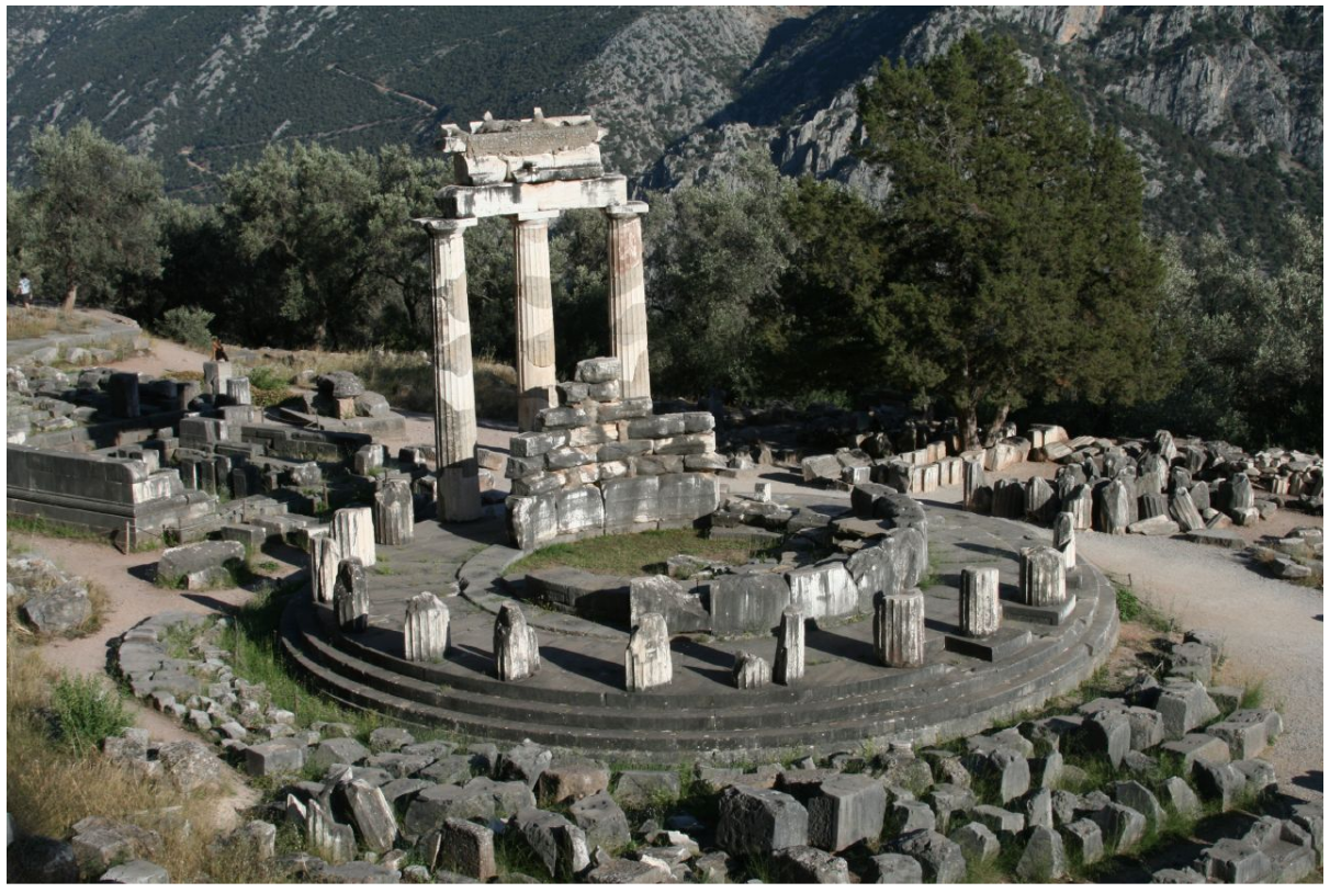
To simplify the construction of a tholos temple, we will divide it into two parts, one creating the base, and another positioning the columns.
For the base, we can consider a set of stacked cylinders to form the circular steps, as shown in this figure. Thus, the base will be composed of \(n\) steps of height \(\Delta h_b\), with a base radius \(r_b\) shrinking \(\Delta r_b\) at each step.
A tholos base section. The base is composed by a sequence of stacked cylinders whose base radius \(r_b\) shrinks \(\Delta r_b\) at each step, and whose height grows in increments of \(\Delta h_b\) at each step.
To draw the bottom cylinder we have to consider its radius and the d_height. To draw the remaining cylinders, we have also to consider the radius decrement d_radius. These steps will be built using a recursive process:
If the number of steps to create is zero, nothing needs to be done.
Otherwise, we place a step (modeled with a cylinder) with the given radius and height and, recursively, we place the remaining steps on its top.
This process is implemented by the following function:
tholos_base(p, n_steps, r_base, dh_base, dr_base) =
if n_steps == 0
nothing
else
cylinder(p, r_base, dh_base)
tholos_base(p+vxyz(0, 0, dh_base),
n_steps-1,
r_base-dr_base,
dh_base,
dr_base)
end
For the positioning of the columns we will also consider a process that, at each step, only places one column at a given position and, recursively, places the remaining columns.
Given its circular structure, the construction of this type of building is simplified by the use of polar coordinates. In fact, we can elaborate a recursive process that, given the peristyle radius \(r_p\) and the initial angle \(\phi\), places a column in that position. Thereafter, it places the remaining columns using the same radius but incrementing \(\phi\) with \(\Delta\phi\), as shown in this figure.
Scheme of the construction of a tholos: \(r_b\) is the base radius, \(r_p\) is the peristyle radius (distance from the center of the columns to the center of the base), \(h_p\) is the peristyle height, \(\phi\) is the initial angle of the columns, and \(\Delta\phi\) is the angle between them.
The angular increment \(\Delta\phi\) is obtained by dividing the circumference by the number \(n\) of columns to place, i.e., \(\Delta\phi=\frac{2\pi}{n}\). The function definition is thus:
tholos_columns(p, n_columns, r_peristyle, phi, dphi, h_peristyle) =
if n_columns == 0
nothing
else
doric_column(p+vpol(r_peristyle, phi), h_peristyle)
tholos_columns(p, n_columns-1, r_peristyle, phi+dphi, dphi, h_peristyle)
end
Finally we define the function tholos that, given the necessary parameters to the two previous functions, invokes them sequentially:
tholos(p, n_steps, rb, dhb, drb, n_columns, rp, hp) =
begin
tholos_base(p, n_steps, rb, dhb, drb)
tholos_columns(p+vxyz(0, 0, n_steps*dhb),
n_columns,
rp,
0,
2*pi/n_columns,
hp)
end
This figure shows the model generated by the evaluation the following expression:
tholos(xyz(0, 0, 0), 3, 7.9, 0.2, 0.2, 20, 7, 4)
A perspective of the Tholos of Delphi, comprising \(20\) Doric columns with a height of \(4\) meters each, placed within a circle with a radius of \(7\) meters.
4.3.2 Exercises 25
4.3.2.1 Question 72
Consider the construction of a tower made of several modules, in which each module has exactly the same characteristics of a tholos, as presented in the figure below:
The top of the tower has a similar shape to the tholos base, although with more steps.
Define the function tholos_tower that, from the center of the tower’s base, the number of modules, the number of steps at the top of the tower, and the remaining necessary parameters to define a module similar to a tholos, builds a tower like the one presented in the previous image, on the left. Test the function by creating a tower with: \(6\) modules, \(10\) steps at the top, \(3\) steps per module, each step with a height and depth of \(0.2\), a base radius of \(7.9\), \(20\) columns per module, a peristyle radius of \(7\) and columns with a height of \(4\) meters.
Based on the previous answer, redefine the tower’s construction so that the radial dimension decreases with the height, as is visible on the center of the previous image.
Based on the previous answer, redefine the tower’s construction so that the number of columns decreases with height, as presented on the right of the previous image.
4.3.2.2 Question 73
In order to see the stereoscopic image, focus your attention on the middle of the two images and cross your eyes, as if you were to focus on a very close object. You will notice that the two images become four, although slightly blurry. Then try to uncross the eyes in order to see only three images, i.e., until the two central images are overlapped. Concentrate on that overlap and let your eyes relax until the image is focused.
Define a function that, starting from the city center and the central cylinders radius, creates a city similar to the presented one.
4.4 Ionic Order
The Ionic order is one of the three classical orders of Greek architecture. The volute, an architectural element that characterizes the Ionic order, is a spiral-shaped ornament placed at the top of an Ionic capital. This figure shows an example of an Ionic capital containing two volutes. Although we still have numerous samples of volutes from antiquity, their drawing process was never clear.
Volutes of an Ionic capital. Photograph by See Wah Cheng.
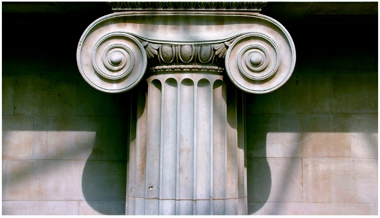
Vitruvius, in his architectural treatise, describes the Ionic volute: a spiral-shaped curve that starts at the base of the abacus, unfolds into a series of turns and joins with a circular element called the eye. Vitruvius describes the spiral drawing process through a composition of arcs, each covering a quarter of a circumference, starting at the outermost point and decreasing the arc radius one at a time, until joining with the eye. In his description, there are still some details to be explained, in particular, the position of the centers of the arcs. Vitruvius mentions that a calculation and a figure will be added at the end of the book, but, unfortunately, those were never found. The doubts regarding the drawing process of this element become even more evident when analysis performed on the many volutes that survived the antiquity revealed differences to the proportions described by Vitruvius.
During the Renaissance period, these doubts made researchers rethink Vitruvius’ method by suggesting personal interpretations or completely new methods for designing volutes. The more relevant methods are the ones proposed in the 16th century by Sebastiano Serlio (based on the composition of semi-circumferences), by Giuseppe Salviati (based on the composition of quarters of a circumference), and by Guillaume Philandrier (based on the composition of eighths of a circumference).
All those methods differ in many details but, generically, they are all based on the use of arcs of circumference with constant angle amplitude but with a decreasing radius. Obviously, to ensure continuity between the arcs, their centers must change as they are being drawn. This figure presents the process of drawing spirals using quarters of a circumference.
Drawing of a spiral using quarters of a circumference.
As shown in the figure above, in order to draw the spiral we must draw successive circumference arcs. The first arc is centered at the point \(P\) and has a radius \(r\). This first arc goes from the angle \(\pi/2\) to \(\pi\). The second arc is centered at the point \(P_1\) and has a radius of \(r\cdot f\), with \(f\) being the reduction factor of the spiral. This second arc goes from the angle \(\pi\) to \(\frac{3}{2}\pi\). An important detail is the relationship between the coordinates of \(P\) and \(P_1\): for the second arc starting point to be coincident with the first arc endpoint, its center must be the sum of \(P\) with the vector \(\vec{v}_0\), whose length is \(r\cdot(1-f)\), and whose direction is equal to the final angle of the first arc.
This process should be repeated for the remaining arcs to calculate the coordinates \(P_2\), \(P_3\), etc., as well as the radii \(r\cdot f \cdot f\), \(r\cdot f \cdot f \cdot f\), etc., which are needed to draw the remaining arcs.
Described this way, the drawing process seems complicated. However, it is possible to rewrite it so that it becomes much simpler, by thinking about the spiral as an arc followed by a smaller spiral. Therefore, a spiral centered at the point \(P\), with a radius \(r\), and an initial angle \(\alpha\), can be defined by an arc of radius \(r\), centered at \(P\), with an initial angle of \(\alpha\) and a final angle of \(\alpha + \frac{\pi}{2}\), followed by a spiral centered at \(P+\vec{v}\), with a radius of \(r\cdot f\) and an initial angle of \(\alpha + \frac{\pi}{2}\). The vector \(\vec{v}\) will have a length of \(r\cdot(1-f)\) and an angle of \(\alpha + \frac{\pi}{2}\).
Obviously, being this a recursive process, it is necessary to define the stopping condition, for which we have (at least) two possibilities:
End when the number of arcs is zero.
End when the radius \(r\) is smaller than a certain limit.
End when the angle \(\alpha\) is bigger than a certain limit.
For now, we will consider the first possibility. According to the described process, let’s define the function that draws the spiral with the following parameters: the p starting point, the r initial radius, the a initial angle, the n number of quarters of a circumference, and the f reduction factor:
spiral(p, r, a, n, f) =
if n == 0
nothing
else
circumference_quarter(p, r, a)
spiral(p+vpol(r*(1-f), a+pi/2), r*f, a+pi/2, n-1, f)
end
Note that the spiral function is recursive, as it is defined in terms of itself. Obviously, the recursive case is simpler than the original case, since the number of quarters of a circumference is smaller, progressively approaching the stopping condition.
To draw each arc we will use Khepri’s arc function which receives the arc’s center, radius, initial angle, and angle amplitude. To visualize the drawing process, we will also draw two lines starting at the arc’s center and ending in its endpoints. Later, once we have finished developing these functions, we will remove them.
circumference_quarter(p, r, a) =
begin
arc(p, r, a, pi/2)
line(p, p+vpol(r, a))
line(p, p+vpol(r, a+pi/2))
end
Now we can test an example:
spiral(xy(0, 0), 3, pi/2, 12, 0.8)
The spiral drawn by the expression above is shown in this figure.
A spiral composed by quarters of a circumference.
The spiral function allows us to define any number of spirals, but with one restriction: each circular arc corresponds to an angle increment of \(\frac{\pi}{2}\). Obviously, this function would be more useful if this increment was also a parameter, as shown in this figure.
Spiral with the angle increment as a parameter.
As can be deduced from observing this figure, the required modifications are relatively simple. We only need to add the parameter da, representing the angle increment \(\Delta_\alpha\) of each arc, and replace the occurrences of \(\frac{\pi}{2}\) with it. Naturally, instead of always drawing a quarter of a circumference, we will now draw an arc of angle amplitude \(\Delta_\alpha\). Since the use of this parameter also affects the meaning of the parameter \(n\), which now represents the number of arcs with that amplitude, it is advisable to explore a different stopping condition based on the intended final angle fa. However, we need to consider one final detail: the last arc may not be a complete arc if the difference between the final and initial angle exceeds the angle amplitude. In this case, the arc will only have this difference as angle amplitude. The new definition is then:
spiral(p, r, a, da, fa, f) =
if fa-a < da
spiral_arc(p, r, a, fa-a)
else
spiral_arc(p, r, a, da)
spiral(p+vpol(r*(1-f), a+da), r*f, a+da, da, fa, f)
end
The function that draws the arc is a generalization of the one that draws one quarter of a circumference:
spiral_arc(p, r, a, da) =
begin
arc(p, r, a, da)
line(p, p+vpol(r, a))
line(p, p+vpol(r, a+da))
end
Right now, to draw the spiral previously represented in this figure, we have to evaluate the following expression:
spiral(xy(0, 0), 3, pi/2, pi/2, pi*6, 0.8)
Noticeably, we can now easily draw other spirals. The spirals produced by the following expressions, comprising different reduction factors, are shown in this figure:
spiral(xy(0, 0), 2, pi/2, pi/2, pi*6, 0.9)
spiral(xy(4, 0), 2, pi/2, pi/2, pi*6, 0.7)
spiral(xy(8, 0), 2, pi/2, pi/2, pi*6, 0.5)
Various spirals with different reduction factors: \(0.9\), \(0.7\) and \(0.5\), respectively.
Note that these are mere approximations. The original methods were much more complex.
spiral(xy(0, 0), 2, pi/2, pi, pi*6, 0.8)
spiral(xy(4, 0), 2, pi/2, pi/2, pi*6, 0.8)
spiral(xy(8, 0), 2, pi/2, pi/4, pi*6, 0.8)
The results of evaluating the previous expressions are shown in this figure.
Various spirals with a reduction factor of \(0.8\) and different angle increments: \(\pi\), \(\frac{\pi}{2}\), and \(\frac{\pi}{4}\), respectively.
Finally, in order to compare the drawing process of the different spirals, we should adjust the reduction factor to the angle increment, so that the reduction is applied to one whole turn and not just to the chosen angle increment. Thus, we have the following expressions:
spiral(xy(0, 0), 2, pi/2, pi, pi*6, 0.8)
spiral(xy(4, 0), 2, pi/2, pi/2, pi*6, 0.8^(1/2))
spiral(xy(8, 0), 2, pi/2, pi/4, pi*6, 0.8^(1/4))
The results of evaluating the previous expressions are shown in this figure.
Various spirals with a reduction factor of \(0.8\) per turn and with different angle increments: \(\pi\), \(\frac{\pi}{2}\) and \(\frac{\pi}{4}\), respectively.
4.4.1 Exercises 26
4.4.1.1 Question 74
The golden spiral is a spiral whose growth factor is the golden ratio \(\varphi\), being \(\varphi=\frac{1 + \sqrt{5}}{2}\). The golden ratio was popularized by Luca Pacioli in his book Divina Proporzione first printed in 1509, although there are numerous accounts of its use many years before.
The following drawing illustrates a golden spiral inscribed in the correspondent golden rectangle, in which the bigger side is \(\varphi\) times bigger than the smaller side.
As can be seen in the previous drawing, the golden rectangle has the remarkable property of being recursively (and infinitely) decomposable into a square and another golden rectangle.
Redefine the spiral_arc function so that, in addition to creating an arc, it also creates the bounding square. Then write an expression that creates the golden spiral represented above.
4.4.1.2 Question 75
An oval is a geometric shape that resembles the outline of birds’ eggs. Given the variety of egg forms in nature, it is natural to consider several oval shapes. The following figure shows some examples in which some of the parameters that characterize the oval are systematically changed:
An oval is composed of four circumference arcs as presented in the following image:
The circular arcs needed to draw the oval are defined by the radii \(r_0\), \(r_1\) and \(r_2\). Note that the circular arc of radius \(r_0\) covers an angle of \(\pi\) and the circular arc of radius \(r_2\) covers an angle of \(\alpha\).
Define the oval function that draws an egg. The function should receive as parameters the coordinates of the point \(P\), the \(r_0\) and \(r_1\) radii, and the egg’s height \(h\).
4.4.1.3 Question 76
Define the cylinder_pyramid function that builds a pyramid of cylinders piled on top of each other, as presented in the following image. Note that the cylinders decrease in size (both in length and radius) and suffer a rotation as they are being piled.
4.5 Recursion in Nature
Recursion is present in countless natural phenomena. A recursive process allows the generation of self-similar patterns (in which the whole has a shape similar to a part of itself). Those patterns are visible in many apparent chaotic structures. Mountains, for example, exhibit irregularities that when observed at an appropriate scale are identical to... mountains. A river has tributaries and each tributary is identical to... a river. A blood vessel has branches and each branch is identical to... a blood vessel. All these natural entities are examples of recursive structures.
A tree is another good example of a recursive structure, since, as it can be seen in this figure, tree branches are similar to small trees growing from the trunk. Likewise, from each tree branch there are other small trees growing from them, a process that repeats itself until its dimension becomes sufficiently small and other structures appear, such as leaves, flowers, fruits, etc.
The recursive structure of trees. Photograph by Michael Bezzina.
If, in fact, a tree has a recursive structure, it should be possible to create trees with recursive functions. To test this theory, let us start by considering a very simplistic version of a tree, where we have a trunk that, at one certain point, is divided into two sub-trunks, or branches. Each of these branches grows with an angle from the main trunk, and reaches a certain length that is a fraction of the main trunk’s length, as shown in this figure. The stopping condition is reached when the length of the branch becomes so small that, instead of continuing dividing itself, a different structure appears. To simplify, let us consider that, at the extremity of the smaller branches, a leaf appears, which we will represent with a small circle.
Drawing parameters of a tree.
Let us consider a tree function that receives, as arguments, the position \(P\) of the tree base, the length \(l\) of the trunk and the angle \(\alpha\) of the trunk. For the recursive case, we will have as parameters the opening angle \(\Delta_\alpha\) that the new branch should make with the previous one, and the reduction factor \(f\) for the trunk’s length.
The first step is to compute the top of the trunk, which can be easily done with polar coordinates, and we draw the trunk from the base to the top. Next, we test if the drawn trunk is sufficiently small. If it is, we finish with the drawing of a circle centered at top. Otherwise, we make one recursive call to draw a sub-tree on the right and another to draw a sub-tree on the left. The definition of the function is then:
tree(p, l, a, da, f) =
let top = p+vpol(l, a)
branch(p, top)
if l < 2
leaf(top)
else
tree(top, l*f, a+da, da, f)
tree(top, l*f, a-da, da, f)
end
end
branch(p0, p1) = line(p0, p1)
leaf(p) = circle(p, 0.2)
A first example of a tree, created by the following code, is presented in this figure.
tree(xy(0, 0), 20, pi/2, pi/8, 0.7)
Drawing of a tree, whose trunk measures \(20\) units, with an initial angle of \(\frac{\pi}{2}\), an opening angle of \(\frac{\pi}{8}\) and a reduction factor of \(0.7\).
Other examples are presented in this figure, in which the opening angle and the reduction factor vary. The sequence of expressions that generated those examples is the following:
tree(xy(0, 0), 20, pi/2, pi/8, 0.6)
tree(xy(100, 0), 20, pi/2, pi/8, 0.8)
tree(xy(200, 0), 20, pi/2, pi/6, 0.7)
Various trees with different opening angles and reduction factors.
Unfortunately, the presented trees are "excessively" symmetrical: in nature it is literally impossible to find perfect symmetries. For this reason, the model should become a little bit more sophisticated, with the introduction of different growth parameters for the branches on the left and on the right. For that, instead of having a single opening angle and only one length reduction factor, we will apply two, as presented in this figure.
Drawing parameters of a tree with asymmetrical growth.
The redefinition of the tree function to receive the additional parameters is straightforward:
tree(p, l, a, da0, f0, da1, f1) =
let top = p+vpol(l, a)
branch(p, top)
if l < 2
leaf(top)
else
tree(top, l*f0, a+da0, da0, f0, da1, f1)
tree(top, l*f1, a-da1, da0, f0, da1, f1)
end
end
This figure presents new examples of trees with different opening angles and reduction factors on the left and right branches, which were generated by the following expressions:
tree(xy(0, 0), 20, pi/2, pi/8, 0.6, pi/8, 0.7)
tree(xy(80, 0), 20, pi/2, pi/4, 0.7, pi/16, 0.7)
tree(xy(150, 0), 20, pi/2, pi/6, 0.6, pi/16, 0.8)
Various trees generated with different opening angles and reduction factors for both left and right branches.
The trees generated by the tree function are only a poor model of reality. Although there are obvious signs that various natural phenomena can be modeled by recursive processes, nature is not as deterministic as our functions. So, in order to make our tree function closer to reality, it is crucial that some randomness is incorporated. This will be the subject of the next section.
5 State
5.1 Introduction
As we have seen, Julia allows us to establish an association between a name and an entity. In this section, we will see that Julia also allows us to change this association. This operation is called assignment and is done through the = operator.
In this section we are going to discuss the concept of assignment. We will start by introducing an important topic where assignment plays a key role: randomness.
5.2 Randomness
Designing involves making conscious decisions that lead to an intended purpose. In this sense, designing appears to be a rational process in which there is no room for randomness, luck, or uncertainty. In fact, so far, all the designs we presented were the result of completely rational processes that were needed because the computer requires a rigorous specification of what is intended, not allowing any ambiguities. However, it is known that architects often have to try different solutions before finding the one that pleases them. So, although the final design may have a structure that reflects the architect’s rational intention, the process that led to this final design is not necessarily rational and may have gone through phases of ambiguity and uncertainty.
When architecture is inspired by nature, an additional factor of randomness arises. In many cases, nature is intrinsically random, however, that randomness is not uncontrolled, having some restrictions. This fact is easily understood when we consider that, although there are no two equal pine trees, we can recognize the pattern that characterizes a pine tree. In all its masterpieces, nature combines regularity and randomness. In some cases, as in the growth of crystals, there is more regularity than randomness. In other cases, as in the behavior of subatomic particles, there is more randomness than regularly.
As in nature, this combination of randomness and regularity is visible in several works of modern architecture. As an example, consider two important works by the architect Oscar Niemeyer: the Itamaraty Palace and the Mondadori Palace, visible in this figure. Despite the clear resemblances between them, the first one excels for the regularity in its arcade, while the second one stands out for its evident randomness.
Two buildings by Oscar Niemeyer: the Itamaraty Palace, designed in 1962 (above), and the Mondadori Palace, designed in 1968 (below). Photographs by Bruno Kussler and Tristan Nitot, respectively.
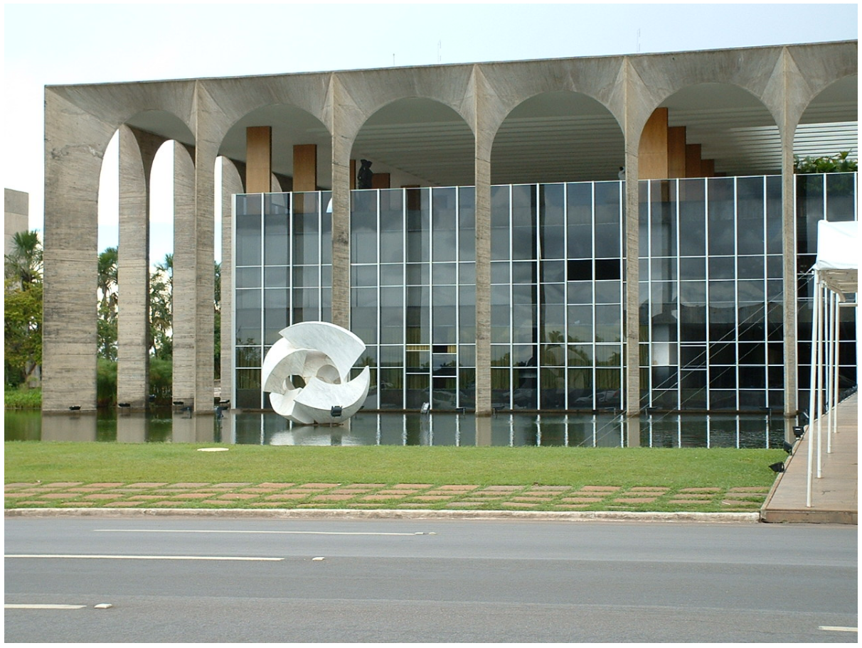
Although the design process involves making conscious and rational decisions, it also encompasses a large amount of intuitive and irrational choices. Design problems often rely on complex and inaccurate information, and design solutions are unpredictable. In this sense, designing has inherently some degree of uncertainty and randomness.
All the designs we presented so far were the result of completely rational processes, since the computer requires a rigorous specification of what is intended, not allowing any ambiguities. However, if we want to use computers to design and the intended design requires randomness, then we must be able to incorporate it in our algorithms. In practice, randomness can be incorporated in various ways, for example:
An object’s color may be chosen randomly.
The length of a wall can be a random value between certain limits.
The decision to divide an area or keep it whole can be random.
The shape of a given architectural element can be chosen randomly.
5.3 Random Numbers
In any of the above cases, we can simulate the intended randomness by using numbers chosen within certain limits.
- To produce a random color, we can randomly generate three numbers representing the RGB values of that color.
RGB stands for Red Green Blue, a model where any color can be seen as the composition of the three additive primary colors (red, green and blue).
To produce a random length, we can generate a random number within that length’s limits.
For a logical decision (such as the one of choosing whether to divide a wall or not), we can emulate tossing a coin by randomly generating either zero or one, and treat zero as heads and one as tails.
For a random choice among a set of alternatives (such as the shape of a given architectural element), we can simply generate a random number between one and the number of alternatives and then choose the one corresponding to the randomly generated number.
These examples show us that the ability to generate a random number within a certain range is sufficient to implement many different random processes.
There are two fundamental processes for generating random numbers. The first one is based on the measurement of physical processes which are intrinsically random, such as electronic noise or radioactive decay. The second process is based on the use of arithmetic functions that, given an initial value (called the seed), produce a sequence of seemingly random numbers, where the generation of each number is based on the previous one. In the first case, we are dealing with a true-random number generator, while in the latter case, we are talking about a pseudo-random number generator. The term pseudo is due to the fact that the generated sequence of numbers is not really random: if we repeat the value of the original seed we will also repeat the sequence of generated numbers.
Although a pseudo-random number generator produces a sequence of numbers that are actually not random, it has two important advantages:
It can be easily implemented using any programming language, not requiring any other additional mechanisms to obtain the randomness source.
It can be useful to detect and correct bugs in our programs. In fact, in order to identify the cause of a bug, it may be necessary to reproduce exactly the same conditions that led to that bug. Besides that, after fixing the bug it is often necessary to rerun the program to make sure that the bug no longer occurs. Unfortunately, when the program’s behavior depends on a truly random sequence of numbers, it is impossible to reproduce the exact same conditions: in the next time we run the program, the sequence of numbers will almost certainly be different.
Therefore, from now on, we will only consider pseudo-random number generators, which we will abusively designate as random number generators. A generator of this kind is characterized by a function \(f\) that, given a certain argument \(x_i\), produces a number \(x_{i+1}=f(x_i)\), apparently unrelated to \(x_i\). The seed of the generator is the element \(x_0\) of the sequence.
What is left now is to find a suitable \(f\) function. For this, and among other qualities, it is required that the numbers generated by \(f\) are equiprobable, i.e., all numbers within a certain range are equally probable to be generated. Moreover, it is also demanded that the period of the generated numbers sequence is as large as possible, i.e., the sequence of numbers only starts to repeat itself after the generation of a large amount of numbers.
Numerous functions with these characteristics have been studied up to now. The most used is called the linear congruential generator function, which has the form:
\[x_{i+1} = (a x_i + b)\bmod m\]
The mathematical operation modulo (\(p\bmod q\)) corresponds to the remainder of the division of the first operand (the dividend \(p\)) by the second operand (the divisor \(q\)), having the same sign as the divisor. In Julia, the same behavior is implemented by the operator %, and by the functions mod and rem.
For example, if we have \(a = 25173\), \(b = 13849\), and \(m = 65536\), and we begin the sequence with an arbitrary seed, for example, \(x_0=12345\), we obtain the following pseudo-random numbers:
Actually, this sequence is not random enough as there is a pattern that repeats itself continuously. Can you discover it?
We can easily confirm these results using Julia:
next_random_number(previous_random_number) =
(25173*previous_random_number+13849)%65536
> next_random_number(12345)
2822
> next_random_number(2822)
11031
> next_random_number(11031)
21180
This approach, however, implies that we can only generate a “random” number \(x_{i + 1}\) if we recall the \(x_i\) number generated immediately before, so that we can provide it as an argument for the next_random_number function. Unfortunately, the moment and the point of the program at which we might need a new random number can occur much later and much further than the moment and the point of the program when the last random number was generated, which substantially complicates the program’s writing. It would be preferable that, instead of having a next_random_number function that depends on the previously generated number \(x_i\), we had a random_number function that did not need the previously generated number to be able to produce the next one. This way, at any point of the program where we might need to generate a new random number, we would only have to invoke the random_number function without having to recall the previously generated number. Starting with the same seed value, we would have:
> random_number()
2822
> random_number()
11031
> random_number()
21180
In the next section we will describe how to define the random_number function.
5.4 State
The random_number function shows a different behavior from the functions we have seen so far. Until now, all the functions we have defined behaved according to the rules of mathematics: given a set of arguments, the function produces results and, more importantly, given the same arguments, the function always produces the same results. For example, regardless of the number of times the factorial function is called, for a given argument, it will always produce the factorial of that argument.
The random_number function is different from the others because, besides not needing any argument, it produces a different result each time it is called.
From a mathematical point of view, a function without parameters is not uncommon: it is precisely what is known as a constant. In fact, just as we write \(\sin \cos x\) to designate \(\sin(\cos(x))\), we can just as well write \(\sin \pi\) to designate \(\sin(\pi())\), where \(\pi\) can be seen as a function without arguments.
From a mathematical point of view, a function that produces different results each time it is called is anything but normal. In fact, according to the mathematical definition of function, this behavior is not possible. And yet, this is precisely the behavior we would like the random_number function to have.
To obtain such behavior, it is necessary to introduce the concept of state. We say that a function has state when its behavior depends on its history, i.e., on its previous calls. The random_number function is an example of a function with state, but there are many other examples in the real world. For example, a bank account has a state that depends on all past transactions. A car’s fuel tank also has a state that depends on the past tank fillings and journeys.
For a function to have history it must have memory, i.e., it must recall past events in order to influence future results. So far, we have seen that the = operator allows us to define associations between names and values. However, what has not yet been discussed is the possibility to modify these associations, i.e., change the value that was associated to a particular name. It is this feature that allows us to include memory in our functions.
In the case of the random_number function, the memory that is important to us is the last random number generated. Thus, suppose we had an association between that number and the name previous_random_number. Initially, this name should be associated with the seed of the random number sequence:
previous_random_number = 12345
Now, we can define a random_number function that, not only uses the last value associated with the name previous_random_number, but also updates this association with the new generated value:
random_number() =
previous_random_number = next_random_number(previous_random_number)
Unfortunately, when we try to use the function, it does not seem to work as intended:
> random_number()
ERROR: UndefVarError: previous_random_number not defined
The result is a consequence of the Julia’s rule that says that whenever a name is assigned to a value inside a function, that name is treated as a local variable, meaning that it is only visible inside the function and, moreover, it is only active while the function is being called. Furthermore, a variable that is local to a function makes a global variable with the same name invisible. This is called shadowing, and we say that the local name shadows the global one, making it inaccessible inside the function.
This rule makes sense in many situations, but not in this one, since it implies that the assignment made does not affect the global name as was intended but, instead, the local one. To make things worse, in this particular case, the assignment depends on the previous value assigned to that same name but, given that this name is treated as a local one, it does not have a value yet, so, it is undefined and cannot be used. That is precisely what the error message is saying.
In order to fix this problem, Julia provides a declaration that allows us to assert that a given name refers to a global definition. We will use that declaration to redefine the random_number function:
random_number() =
global previous_random_number = next_random_number(previous_random_number)
Using this definition, the function has the intended behavior.
> random_number()
2822
> random_number()
11031
As we can see, every time the random_number function is called, the value associated with the previous_random_number is updated, influencing the function’s future behavior. Obviously, at any given moment, we can restart the sequence of random numbers simply by restoring the seed value:
> random_number()
21180
> random_number()
42629
> previous_random_number = 12345
12345
> random_number()
2822
> random_number()
11031
> random_number()
21180
5.5 Random Choices
Observing the next_random_number function definition, we find that its last operation is computing the remainder of the division by \(65536\), which implies that the function always produces values between \(0\) and \(65535\). Although (pseudo) random, these values are contained in a range that will rarely be useful, as it is much more frequent that we need random numbers that are contained in much smaller intervals. For example, if we want to simulate the action of flipping a coin, we are only interested in randomly generating the numbers \(0\) or \(1\), representing “heads” or “tails”.
Just as our random_number function is limited to the range \([0,65536[\) by the remainder of the division by \(65536\), we can apply the same operation to produce smaller ranges. Therefore, in the case of flipping a coin, we can simply use the random_number function to generate a random number and then compute the remainder of its division by \(2\). Generalizing, when we want random integer numbers in an interval \([0,x[\), we apply the remainder of the division by \(x\). Thus, we can define a new function that generates a random number between zero and a parameter, which we will call random:
random(x) = random_number()%x
In fact, the argument of the random function should be fairly below the limit of the random function to maintain the equiprobability of the results.
It is now possible to simulate a number of random phenomena such as, for example, flipping a coin:
heads_or_tails() = random(2) == 0 ? "heads" : "tails"
Unfortunately, when repeatedly tested, our function does not seem very random:
> heads_or_tails()
"tails"
> heads_or_tails()
"heads"
> heads_or_tails()
"tails"
> heads_or_tails()
"heads"
> heads_or_tails()
"tails"
> heads_or_tails()
"heads"
In fact, the results we are getting are a constant repetition of the pair: heads/tails, which reveals that the expression random(2) merely generates the following sequence:
0101010101010101010101010101010101010101010101010101010101
The same phenomenon occurs for other intervals: for example, the expression random(4) should generate a random number from the set \(\{0,1,2,3\}\), but its repeated invocation generates the following sequence of numbers:
0123012301230123012301230123012301230123012301230123012301
Despite the numbers are perfectly equiprobable, they are clearly not random.
The problem in both previous sequences is the fact that they have a very small period. The period is the number of elements that are generated before the sequence enters into a cycle and starts repeating the same elements previously generated. Obviously, the greater the period, the better the random numbers generator will be. In that sense, the random number generator we have shown is of poor quality.
Great amounts of effort have been invested on finding good random number generators and, although the better ones are produced using fairly more sophisticated methods than the ones we have used so far, it is also possible to find a good linear congruential generator as long as we wisely choose the parameters. In fact, the linear congruential generator \[x_{i+1} = (a x_i + b) \bmod m\] can be a good pseudo-random generator as long as we have \(a=16807\), \(b=0\) and \(m=2^{31}-1=2147483647\). A direct translation of this mathematical definition to Julia produces the following function:
next_random_number(previous_random_number) =
(16807*previous_random_number)%2147483647
Using this new definition, the repeated evaluation of the random(2) expression produces the following sequence:
01001010001011110100100011000111100110110101101111000011110
and the repeated evaluation of the random(4) expression produces:
21312020300221331333233301112313001012333020321123122330222
It is fairly clear that the generated sequences now have a period large enough for any repetition pattern to be detected. Thus, from now on, this is the definition of the next_random_number function that will be used.
5.5.1 Random Fractional Numbers
The process of generating random numbers previously implemented is only able to generate random integer numbers. However, we often need to generate fractional random numbers in an arbitrary interval \([0, x[\), for example \([0, 1[\), which would generate numbers such as 0.05, 0.0123, etc.
This function uses the isa Julia’s function that tests whether an element is of a given type, such as integer numbers (which are represented by Int).
random(x) =
x isa Int ? rem(random_number(), x) : x*random_number()/2147483647.0
We can now apply the random function to produce either integer or real numbers:
> random(1)
0
> random(1.0)
0.34854938618305575
Given its utility, the random function is already predefined in Khepri.
5.5.2 Random Numbers within a Range
Sometimes, instead of generating random numbers in the range \([0, x[\), we prefer to generate random numbers in the range \([x_0, x_1[\). In this case, we just have to generate a random number within \([0, x_1-x_0[\) and then add \(x_0\). The random_range function implements this behavior:
random_range(x0, x1) = x0+random(x1-x0)
Like the random function, the random_range function also produces a real value when any of the limits is a real number. The random_range function is also predefined in Khepri.
As an example, let us reconsider the tree function that models a tree, defined in section the Recursion in Nature as:
tree(p, l, a, da0, f0, da1, f1) =
let top = p+vpol(l, a)
branch(p, top)
if l < 2
leaf(top)
else
tree(top, l*f0, a+da0, da0, f0, da1, f1)
tree(top, l*f1, a-da1, da0, f0, da1, f1)
end
end
To incorporate some randomness in this tree model, we can consider that both the branches’ opening angles and length reduction factors can vary throughout the recursion process. Thus, instead of worrying about having different opening angles and factors for the left and right branches, we will simply have random variations on both sides:
tree(p, l, a, min_a, max_a, min_f, max_f) =
let top = p+vpol(l, a)
branch(p, top)
if l < 2
leaf(top)
else
tree(top,
l*random_range(min_f, max_f),
a+random_range(min_a, max_a),
min_a,
max_a,
min_f,
max_f)
tree(top,
l*random_range(min_f, max_f),
a-random_range(min_a, max_a),
min_a,
max_a,
min_f,
max_f)
end
end
Using this new version, we can generate several similar trees yet sufficiently different to seem much more natural. The trees shown in this figure were generated using exactly the same parameters:
tree(xy(0, 0), 20, pi/2, pi/16, pi/4, 0.6, 0.9)
tree(xy(150, 0), 20, pi/2, pi/16, pi/4, 0.6, 0.9)
tree(xy(300, 0), 20, pi/2, pi/16, pi/4, 0.6, 0.9)
tree(xy(0, 150), 20, pi/2, pi/16, pi/4, 0.6, 0.9)
tree(xy(150, 150), 20, pi/2, pi/16, pi/4, 0.6, 0.9)
tree(xy(300, 150), 20, pi/2, pi/16, pi/4, 0.6, 0.9)
Various trees created with the branches’ opening angles varying in the interval \([\frac{\pi}{16},\frac{\pi}{4}[\) and the length reduction factors varying in the interval \([0.6,0.9[\).
5.5.3 Exercises 27
5.5.3.1 Question 77
The trees produced by the tree function are unrealistic because they are completely two-dimensional, with branches that are simple lines and leaves that are small circles. The calculation of the branches and leaves’ coordinates is also two-dimensional, relying on polar coordinates specified by the length and angle parameters.
Redefine the branch, leave and tree functions in order to increase the realism of the generated trees.
To simplify, assume that the leaves can be simulated by small spheres and that the branches can be simulated by truncated cones with the base radius being \(10\%\) of the branch’s length and the top radius being \(90\%\) of the base radius.
For the generation of trees to be truly three-dimensional, redefine the tree function so that the top of each branch is a point in spherical coordinates chosen randomly from the base of the branch. This implies that the tree function’s parameters of the polar coordinates (length and angle) will have to be replaced by the parameters of the spherical coordinates (length, longitude and colatitude). Therefore, instead of receiving the four limits for generating random lengths and angles, the tree function will receive six limits for generating random lengths, longitudes and colatitudes.
Try different arguments in your redefinition of the tree function, in order to create something similar to the image below:
5.5.3.2 Question 78
Define a function named random_cylinder that receives as argument a number of cylinders \(n\), generating as a result \(n\) cylinders placed in random positions, with random radii and lengths, as presented in the following image:
5.5.3.3 Question 79
A random walk is a formalization of an object motion that is subject to impulses of random magnitude and direction. This phenomenon happens, for example, to a grain of pollen when falling into water: as the molecules of water bump into the grain, it will randomly move.
The following image present three random walks:
Consider a model of a random walk in a two-dimensional plane. Define the random_walk function that has as parameters the starting point \(P\) of the walk, the maximum distance \(d\) the object can move when impulsed, and the \(n\) number of successive impulses the object will receive. Note that, on each impulse, the object moves in a random direction, with a random distance between zero and the maximum distance.
This function should simulate the corresponding random walk, as presented in the previous figure, which was created with three different executions of this function. From left to right, the following parameters were used: \(d=5\) and \(n=100\); \(d=2\) and \(n=200\); and \(d=8\) and \(n=50\).
5.5.3.4 Question 80
Define a biased heads_or_tails function such that, even though it randomly produces the strings "heads" or "tails", the "heads" string falls, on average, only \(30\%\) of the times the function is executed.
5.5.3.5 Question 81
Define the cylinder_sphere function that, given a point \(P\), a length \(l\), a radius \(r\), and a number \(n\), creates \(n\) cylinders, of length \(l\) and radius \(r\), with the base centered at the point \(P\) and with the top positioned randomly, as presented in the following image:
5.5.3.6 Question 82
Define a function called connected_blocks that builds a cluster of connected blocks, i.e., blocks are linked together, as presented in the following figure:
Note that the adjacent blocks always have orthogonal orientations.
5.6 Urban Design
Cities are a good example of the combination between regularity and randomness. Although many ancient cities appear to be chaotic, as a result of their unplanned development, others already encompassed a structured plan, in order to facilitate their growth and improve their living environment. In fact, there are well-known examples of planed cities dating from 2600 BC.
Despite the variety of approaches, the two most usual ways of planning a city are through the orthogonal plan or the circular plan. In the orthogonal plan, straight streets make right angles between them. In the circular plan, the main streets are radial, converging into a central square, whereas the secondary streets are concentric circles around this main square, following the city’s growth. In this section we will explore randomness to simulate cities that follow an orthogonal plan. A good example of a city mainly developed according to this plan is shown in this figure.
Aerial view of New York City. Photograph by Art Siegel.
In an orthogonal plan, the city is organized into blocks. Each block assumes a rectangular or square shape and contains several buildings. To simplify, we will assume that each block has a square shape with fixed size and contains a single building with a fixed height that occupies the entire block. The buildings are separated from each other by streets with a fixed width. The model of this city is presented in this figure.
Scheme of an orthogonal city plan.
In order to structure the function that creates a city with an orthogonal plan, we will first decompose the process into the construction of the successive rows of buildings. Then, the construction of each row of buildings is further decomposed in the successive construction of buildings. Thus, we must parametrize the function based on the number of rows and on the number of buildings per row. In addition, we will need to know the city’s origin point \(P\), the length \(l\) and height \(h\) of each building, and, finally, the width \(s\) of each street. The function will first create a row of buildings separated by streets and then, recursively creates the rest of the city. To simplify this process, we will assume that streets are aligned with the \(X\) and \(Y\) axes, whereby each new row corresponds to a displacement along the \(Y\) axis and each new building corresponds to a displacement along the \(X\) axis. Thus, we will have:
city(p, n, m, l, h, s) =
if n == 0
nothing
else
buildings(p, m, l, h, s)
city(p + vy(l + s),
n - 1, m, l, h, s)
end
For the construction of a row of buildings, the process is the same: we place a building at the starting location and, then, we recursively place the remaining buildings at the next location. The following function implements this process:
buildings(p, m, l, h, s) =
if m == 0
nothing
else
building(p, l, h)
buildings(p + vx(l + s),
m - 1, l, h, s)
end
Finally, we need to define a function that creates a building. To simplify, we will model each building as a parallelepiped:
building(p, l, h) = box(p, l, l, h)
With these three functions we can now try to build a small city. For example, the following expression creates a set of ten rows of buildings with ten buildings per row:
city(xyz(0, 0, 0), 10, 10, 100, 400, 40)
The result is presented in this figure.
An urban area with an orthogonal plan, containing one hundred buildings with the same height.
However, the generated urbanization lacks some of the randomness that typically characterizes cities. To incorporate some randomness, we we will consider that the buildings’ height can randomly vary from a maximum height to one-tenth of that height. This behavior was implemented in a new definition of the building function:
building(p, l, h) = box(p, l, l, random_range(0.1, 1.0)*h)
Using the exact same parameters as before in two consecutive calls of the building function, we can now generate more appealing cities, as shown in this figure and this figure.
An urban area with an orthogonal plan, containing one hundred buildings with random heights.
An urban area with an orthogonal plan, containing one hundred buildings with random heights.
5.6.1 Exercises 28
5.6.1.1 Question 83
The cities produced by the previous functions do not present sufficient variability, as all the buildings have the same shape. To solve this issue, define different functions for different types of buildings: the building0 function should build a parallelepiped with random height (as before), and the building1 function should build a cylindrical tower with a random height (also varying from 10% to 100% of a maximum height), contained within the limits of a block. Then, use both building0 and building1 functions to redefine the building function, so that it randomly generates different buildings. The resulting city should be composed of \(20\%\) circular towers and \(80\%\) rectangular buildings, as illustrated in the following figure:
5.6.1.2 Question 84
The cities created in the previous exercise only allow the creation of two types of buildings: rectangular or cylindrical. However, when we observe a real city, as the one shown in this figure, we find out that there are buildings with many other shapes. This means that, in order to increase the realism of our simulated cities, we need to implement a larger number of functions, each one creating a different kind of building.
View of Manhattan. Photograph by James K. Poole.
Fortunately, a careful observation of this figure shows that, in fact, many of the buildings follow a pattern that can be modeled by stacking successively smaller parallelepipeds with random dimensions. This is something that we can easily implement with a single function.
Consider that such buildings are parametrized by the number of intended blocks to stack, the coordinates of the first block and the length, width and height of the building. The base block has exactly the specified length and width but its height should range between \(20\%\) and \(80\%\) of the total height. The remaining blocks are centered on the block immediately below, with a length and width ranging between \(70\%\) and \(100\%\) of the corresponding parameters of the block immediately below. The height of these blocks should range between \(20\%\) and \(80\%\) of the remaining height of the building. The following image shows some examples of buildings that follow this model:
Based on this specification, define the building_blocks function and use it to redefine the building0 function, so that the generated buildings have a random number of stacking blocks, ranging between \(1\) and \(6\). With this redefinition, the city function should be able to generate a model similar to the following image:
5.6.1.3 Question 85
Typically, cities have an area of relatively tall buildings, which is called business center (abbreviated to CBD, an acronym of Central Business District). As we move away from this area, the height of the buildings tends to decrease, as is visible in this figure.
The variation of the buildings height can be modeled by several mathematical functions but, in this exercise, we intent to apply the two-dimensional Gaussian distribution, given by:
\[f(x,y) = e^{-\left( (\frac{x-x_o}{\sigma_x})^2 + (\frac{y-y_o}{\sigma_y})^2\right)}\]
In the previous formula, \(f\) is the weighting height factor, \((x_0\) and \(y_0)\) are the coordinates of the highest point of the Gaussian surface, and \(\sigma_0\) and \(\sigma_1\) are the factors that determinate the two-dimensional stretch of this surface. In order to simplify, assume that the highest point of the business center is located at the position \((0,0)\) and that \(\sigma_x=\sigma_y=25 l\), with \(l\) being the building’s length. The following image shows an example of one such city:
Incorporate this distribution in the city generation process to produce more realistic cities.
5.6.1.4 Question 86
Cities often have more than one center of tall buildings. These centers are separated from each other by zones of smaller buildings. As in the previous exercise, each area of buildings can be modeled by a Gaussian distribution. Assuming that the multiple areas are independent from each other, the buildings’ height can be controlled by the overlapping of Gaussian distributions, i.e., at each point, the buildings’ height is the maximum height of the Gaussian distributions of the different areas.
Use the previous approach to model a city with three areas of “skyscrapers”, similar to the one presented in the following image:
5.6.1.5 Question 87
It is intended to create a set of \(n\) tangent spheres to a virtual sphere centered at \(P\), with a limit radius \(r_l\). The spheres are centered at a random distance of \(P\), which corresponds to a random value between an inner radius \(r_i\) and an outer radius \(r_o\), as presented in the following scheme:
Define a function called spheres_in_sphere that, from the center \(P\), the radii \(r_i\), \(r_o\), and \(r_l\), and a number \(n\), creates a set of \(n\) spheres, similar to the ones in the following image:
6 Data Structures
6.1 Introduction
Most functions defined in the previous sections aim at producing specific geometric shapes. In this section, we will address functions that aim at creating abstract geometric shapes, in the sense of being represented by a set of positions in space. For example, a polygonal line can be represented by the sequence of positions through which it passes. That sequence can, however, be used for various other purposes, such as creating a sequence of spheres located at those positions or defining the trajectory of a tube passing through those positions. These examples show that the way we manipulate these sets of positions is independent from their subsequent use.
In order to manage sets of positions as a whole, it is necessary to group them in what is called a data structure: a particular arrangement of data that allows it to be treated as a whole. For example, a phone book can be perceived as a data structure that establishes associations between names and phone numbers.
6.2 Arrays
One of the most important data structures that we will discuss is the array. An array is a collection of elements, arranged in a particular way. There are several types of arrays; the most common are one-dimensional arrays (also called vectors) and bi-dimensional arrays (also called matrixes). Bi-dimensional arrays usually arrange elements in rows and columns, as shown below:
\[\begin{bmatrix} a_{11} & a_{12} & \cdots & a_{1n}\\ a_{21} & a_{22} & \cdots & a_{2n}\\ \vdots & \vdots & \ddots & \vdots\\ a_{m1} & a_{m2} & \cdots & a_{mn} \end{bmatrix}\]
As can be seen in the previous description, in order to specify a particular element of an array, one has to provide a sequence of indexes. For example, \(a_{12}\) is the element located in the first row, second column, which, in Julia, is written as a[1,2]. The number of indexes required depends on the dimension of the array; in the above example, the array is bi-dimensional and, thus, it requires two indexes.
Julia provides a specific syntax to create arrays and also numerous operations to deal with them. In the next section, we will focus on one particular kind of array: the one-dimensional array, also called vector.
6.2.1 One-dimensional Arrays
Although arrays can have as many dimensions as we want, it is common to use arrays with just one dimension. A one-dimensional array is also called a vector and, in Julia, it is considered a column vector (since elements are arranged in a single column):
\[\begin{bmatrix} a_{1}\\ a_{2}\\ \vdots\\ a_{n} \end{bmatrix}\]
In Julia, we can build an array by enclosing the elements, separated by a comma, in square brackets:
> numbers = [7, 2, 4, 5]
4-element Array{Int64,1}:
7
2
4
5
Given that this type of array has only one dimension, accessing one of its elements requires only one index. In Julia, the index is provided right after a list, enclosed in square brackets. The last element can be accessed using the special index end. Here is an interaction with Julia illustrating the use of indexes in one-dimensional arrays:
> numbers = [7, 2, 4, 5]
4-element Array{Int64,1}:
7
2
4
5
> numbers[2]
2
> numbers[4]
5
> numbers[end]
5
> numbers[end-1]
4
Another important operation with arrays is the concatenation. It allows us to join the elements of two (or more) arrays. This can be done with the ellipsis operator ... (also called the splat operator):
> more_numbers = [3, 9]
2-element Array{Int64,1}:
3
9
> [numbers..., more_numbers...]
6-element Array{Int64,1}:
7
2
4
5
3
9
> [7, more_numbers...]
3-element Array{Int64,1}:
7
3
9
Note that the ellipsis operator incorporates the elements of an existing array into the new array being created. Without the ellipsis operator, the entire array becomes itself an element of the new array, as is visible in the following interaction:
> [7, more_numbers]
2-element Array{Any,1}:
7
[3, 9]
Julia supports arrays of arrays to an indefinite number of levels, for example: [1, 2, [3, [4], 5], [[[6], 7]], 8].
To “decompose” arrays, Julia provides the concept of slice. An array slice is a section of an array (called subarray), specified by a range of indexes, i.e., a starting and an ending index. Consider the following examples:
julia> numbers[1:3]
3-element Array{Int64,1}:
7
2
4
julia> numbers[2:end]
3-element Array{Int64,1}:
2
4
5
julia> numbers[2:end-1]
2-element Array{Int64,1}:
2
4
julia> numbers[2:2]
1-element Array{Int64,1}:
2
julia> numbers[2:1]
0-element Array{Int64,1}
In the last example, the result is an empty array. This array can also be created by simply writing []. For instance, we have:
> numbers[2:1] == []
true
6.3 Recursion over Arrays
It should be clear that an array slice is still an array. This fact provides an interesting point of view over arrays: they are a recursive data type. If we slice an array from index 2 till its end, we obtain a slightly smaller version of the same array, only lacking the first element. This is visible in the example below:
> students = ["John", "Peter", "Mary"]
3-element Array{String,1}:
"John"
"Peter"
"Mary"
> students[2:end]
2-element Array{String,1}:
"Peter"
"Mary"
This means we can decompose an array into its first element and its remaining elements:
> students == [students[1], students[2:end]...]
true
This also means that we can successively reduce an array by computing its slice from the second element to the end, until we get an empty array:
> students = students[2:end]
2-element Array{String,1}:
"Peter"
"Mary"
> students = students[2:end]
1-element Array{String,1}:
"Mary"
> students = students[2:end]
0-element Array{String,1}
This means that an array can be described by a recursive definition, where the array concept is described in terms of itself:
If an array has no elements, it is an empty array;
Otherwise, the array is composed by one element followed by a slightly smaller array.
Notice that, in the previous definition, the stopping condition is the empty array.
One of the interesting properties of recursive types is that operations that deal with elements of recursive type can be implemented by recursive functions. For example, to define a function that tells us how many elements an array has, we can think recursively:
If the array is empty, the number of elements is zero.
Otherwise, the number of elements is one plus the number of elements of the rest of the array
To ensure the correctness of our reasoning, we must guarantee that the requirements of a proper recursive definition are satisfied, namely:
There is a reduction of the problem’s complexity in every recursive invocation: in fact, in each recursive invocation the array becomes smaller.
There is a simplest case where the answer is immediate: when the array is empty, the number of elements is zero.
The result of the recursion is used to respond to the original problem: it is true that the number of elements in an array is the same as adding \(1\) to the number of elements in that array without the first element.
Translating the previous recursive definition into Julia, we get the following function:
number_of_elements(array) =
array == [] ? 0 : 1+number_of_elements(array[2:end])
Here are two examples of the use of the function:
> number_of_elements([1, 2, 3, 4])
4
> number_of_elements([])
0
It is important to note that the presence of subarrays is irrelevant for the computation of the number of elements in an array: each subarray is just an element of the array and, thus, counts as one. For example:
> number_of_elements([[1, 2], [3, 4, 5, 6]])
2
As we can see in the previous example, the array only contains two elements, despite each element being an array with more elements.
Finally, it is important to know that Julia provides the predefined function length that does the same as the function number_of_elements in a much more efficient way. An example of its use is shown below:
> length([1, 2, 3, 4])
4
6.3.1 Exercises 29
6.3.1.1 Question 88
Define a delete_nth function that receives a number \(n\) and an array, and deletes the \(n\)th element of the array.
Consider the following example of the function usage:
> delete_nth(2, [1, 2, 3, 4, 5])
4-element Array{Int64,1}: 1 3 4 5
6.3.1.2 Question 89
Write a function that, given an array, returns a randomly selected element of that array.
6.3.1.3 Question 90
Define the one_of_each function that, given an array of arrays, creates an array containing a random element of each array, in the same order. For example:
> one_of_each([[0, 1, 2], [3, 4], [5, 6, 7, 8]])
3-element Array{Int64,1}: 1 3 7
> one_of_each([[0, 1, 2], [3, 4], [5, 6, 7, 8]])
3-element Array{Int64,1}: 1 4 8
> one_of_each([[0, 1, 2], [3, 4], [5, 6, 7, 8]])
3-element Array{Int64,1}: 2 3 5
6.3.1.4 Question 91
Define the random_elements function that, given a number \(n\) and an array, returns \(n\) elements of the array picked randomly. For example:
> random_elements(3, [0, 1, 2, 3, 4, 5, 6])
ERROR: BoundsError: attempt to access 5-element Array{Int64,1} at index [6] Stacktrace: [1] getindex(::Array{Int64,1}, ::Int64) at ./array.jl:731 [2] random_elements(::Int64, ::Array{Int64,1}) at ./none:6 (repeats 3 times)
6.3.1.5 Question 92
Define the reverse function that, given an array, returns an array containing the same elements but in reverse order.
6.3.1.6 Question 93
Given that arrays are flexible data structures, we often use arrays containing other arrays that, in turn, may contain other arrays, and so on. That is the case, for example, of the arrays [[1, 2], [3, 4]] and [[[1, 2], [3, 4], [5, 6]], [[7, 8], [9, 0]]]
Write a function called flatten that receives an array as argument, possibly containing other arrays, and returns another array with all the elements of the original array, in the same order, but without any subarrays, for example:
> flatten([1, 2, [3, 4, [5, 6]], 7])
flatten (generic function with 1 method)
6.4 Enumerations
We saw that arrays can be sliced using a range of indexes, starting at a number and ending in another. The range of indexes represents all integers between those two limits. The elements in a range can be enumerated, by considering that, given the limits \(a\) and \(b\) of an interval \([a, b]\) and an increment \(i\), we obtain an array containing the numbers \(a\), \(a+i\), \(a+2i\), \(a+3i\), \(a+4i\), ..., up to \(a+ni \geq b\).
We can take advantage of recursion to implement this idea: the enumeration of the numbers in the interval \([a, b]\) with an \(i\) increment is exactly the same as the number \(a\) followed by the enumeration of the numbers in the interval \([a + i, b]\). If we repeat this process a sufficient number of times, we reach the simplest case of all: an enumeration in the interval \([a, b]\) wherein \(a>b\), whose result is an empty array.
This description can now be translated into the function’s definition:
enumerate(a, b, i) = a > b ? [] : [a, enumerate(a+i, b, i)...]
As an example:
> enumerate(1, 5, 1)
5-element Array{Int64,1}: 1 2 3 4 5
> enumerate(1, 5, 2)
3-element Array{Int64,1}: 1 3 5
To make the function even more generic, we should also cover the case where \(i\) is a negative increment, which is useful, for example, for a regressive counting.
The current definition of the enumerate function does not support regressive counting, because the use of a negative increment causes infinite recursion. The problem lies in the stopping condition: the operator > is only suitable for the case in which the increment is positive. When the increment is negative, we should use <. So, to solve this problem, the function must identify the correct enumeration to use:
enumerate(a, b, i) =
begin
enumerate_up(a) = a > b ? [] : [a, enumerate_up(a+i)...]
enumerate_down(a) = a < b ? [] : [a, enumerate_down(a+i)...]
i > 0 ? enumerate_up(a) : enumerate_down(a)
end
Now we can have:
> enumerate(1, 5, 1)
5-element Array{Int64,1}: 1 2 3 4 5
> enumerate(5, 1, -1)
5-element Array{Int64,1}: 5 4 3 2 1
> enumerate(6, 0, -2)
4-element Array{Int64,1}: 6 4 2 0
The function enumerate describes an operation that is so common that Julia already provides support for it: the expression start:step:stop represents an enumeration. When the increment "step" is one, it can be omitted. To collect the elements of an enumeration in an array, we can use the function collect:
julia> collect(1:2:4)
2-element Array{Int64,1}:
1
3
julia> collect(1:4)
4-element Array{Int64,1}:
1
2
3
4
6.4.1 Exercises 30
6.4.1.1 Question 94
The \(iota\) function is an enumeration starting at \(0\) and ending at the upper limit \(n\), excluding the \(n\) value, containing the elements of the enumeration separated by a given increment. For example:
> iota(10, 1)
10-element Array{Int64,1}: 0 1 2 3 4 5 6 7 8 9
> iota(10, 2)
5-element Array{Int64,1}: 0 2 4 6 8
Define the iota function using the enumerate function.
6.4.1.2 Question 95
Define a function called ismember that receives a number and an array, and then checks whether that number exists in the given array. Here are two examples of the use of the function:
> ismember(3, [5, 2, 1, 3, 4, 6])
true
> ismember(7, [5, 2, 1, 3, 4, 6])
false
6.4.1.3 Question 96
Define the function eliminate1 that receives a number and an array, and returns an identical array without the first occurrence of that number. Here is an example:
> eliminate1(3, [1, 2, 3, 4, 3, 2, 1])
6-element Array{Int64,1}: 1 2 4 3 2 1
6.4.1.4 Question 97
Define a function called eliminate that receives a number and an array, and returns an identical array without any occurrence of that number. Here is an example:
> eliminate(3, [1, 2, 3, 4, 3, 2, 1])
5-element Array{Int64,1}: 1 2 4 2 1
6.4.1.5 Question 98
Define a function called replace that receives two numbers and an array, and returns an identical array with all the occurrences of the second argument replaced with the first argument. Here is an example:
> replace(0, 1, [1, 2, 1, 3])
4-element Array{Int64,1}: 0 2 0 3
> replace(0, 1, [2, 3, 4, 5])
4-element Array{Int64,1}: 2 3 4 5
6.4.1.6 Question 99
Define a function called remove_duplicates that, given an array of numbers, returns an identical array without the repeated numbers. Here is an example:
> remove_duplicates([1, 2, 3, 3, 2, 4, 5, 4, 1])
5-element Array{Int64,1}: 3 2 5 4 1
6.4.1.7 Question 100
Define a function called occurrences that, from a number and an array, returns the number of times that number appears in the array. Here is an example:
> occurrences(4, [1, 2, 3, 3, 2, 4, 5, 4, 1])
2
6.4.1.8 Question 101
Define a function called position that receives a number and an array as arguments and returns the position of the first occurrence of the number in the array. Note that positions in an array start at one. For example:
> position(4, [1, 2, 3, 3, 2, 4, 5, 4, 1])
6
6.5 Polygons
Arrays are particularly useful to represent abstract geometrical entities, i.e., entities about which we are only interested in knowing certain properties, such as their position. In that case, we can use an array of positions, i.e., an array in which the elements represent positions in space.
As an example, imagine we want to represent a polygon. By definition, a polygon is a plane figure bounded by a closed path composed by a sequence of line segments. Each line segment is an edge (or side) of the polygon. Each point where two line segments meet is a vertex of the polygon.
Based on this definition, it is easy to infer that one of the simplest ways to represent a polygon is through a sequence of positions indicating the positions of the vertices by the order we should connect them, admitting the last element is connected to the first one. It is precisely this sequence of arguments that we provide in the following example of the Khepri’s polygon function (see the Bi-dimensional Drawing section):
polygon(xy(-2, -1), xy(0, 2), xy(2, -1))
polygon(xy(-2, 1), xy(0, -2), xy(2, 1))
The result of evaluating these expressions is shown in this figure.
Two overlapping polygons.
Now, let us suppose that, rather than explicitly indicate each vertex position, we want a function to produce that same sequence of positions. For this, the use of arrays constitutes a valuable help, since they allow the representation of sequences. Moreover, many of the geometric functions, such as line and polygon, accept arrays as argument. In fact, this figure can be reproduced by the following expressions:
polygon([xy(-2, -1), xy(0, 2), xy(2, -1)])
polygon([xy(-2, 1), xy(0, -2), xy(2, 1)])
In the same way that a triangle can be represented by an array with three vertices, a quadrilateral can be represented by an array with four vertices, an octagon can be represented by an array with eight vertices, a triacontakaihenagon can be represented by an array with thirty-one vertices, and so on. In the next sections we will focus on how to create these arrays.
6.5.1 Regular Stars
The pentagram was the symbol of mathematical perfection for the Pythagoreans, the symbol of the supremacy of the spirit over the four elements of matter for the occultists, and the symbol of the Five Holy Wounds of Christ for the Christians. The pentagram was also associated with the proportions of the human body, and has been used by the Freemasonry and, when inverted, by Satanic cults.
Variations of star polygons in a window of the Amber Fort, located in the district of Jaipur, India. Photograph by David Emmett Cooley.
Apart from the symbolic connotations, the pentagram is, first of all, a polygon. For this reason, it can be drawn by the polygon function, as long as we produce an array with the positions of its vertices. To that end, we will now focus on this figure, where we see that the five pentagram vertices divide the circle into 5 parts with arcs measuring \(\frac{2\pi}{5}\) each. From the pentagram’s center, its top vertex makes an angle of \(\frac{\pi}{2}\) with the \(X\) axis. This top vertex must then be connected, not with the next vertex, but with the one immediately after it, i.e., the one corresponding to a rotation of two arcs or \(\frac{2\cdot 2\pi}{5}=\frac{4}{5}\pi\). We can now define the pentagram_vertices function that creates the array of vertices of the pentagram:
pentagram_vertices(p, r) =
[p+vpol(r, pi/2+0*4/5*pi),
p+vpol(r, pi/2+1*4/5*pi),
p+vpol(r, pi/2+2*4/5*pi),
p+vpol(r, pi/2+3*4/5*pi),
p+vpol(r, pi/2+4*4/5*pi)]
Creation of a pentagram.
It is clear that the pentagram_vertices function contains a lot of repetitive code, so we need to find a more structured way of generating the pentagram vertices. As before, we could use recursion but, when the goal is the generation of an array of elements where each element can be described by a formula, as it happens with the pentagram_vertices function, it is possible to use a simpler approach, inspired on the syntax used in mathematics to specify array comprehensions. Using array comprehensions, the pentagram_vertices can be written as:
pentagram_vertices(p, r) =
[p + vpol(r, pi/2 + i*4/5*pi)
for i in [0, 1, 2, 3, 4]]
In the previous definition, the array of positions is created from a calculation involving the variable \(i\), in which \(i\) successively takes on each value in the array [0, 1, 2, 3, 4]. We can further simplify the function by using ranges. As previously discussed, a range allows us to represent an array of consecutive numbers as a pair containing the first and last number:
pentagram_vertices(p, r) =
[p + vpol(r, pi/2 + i*4/5*pi)
for i in 0:4]
Although the pentagram_vertices function is only capable of producing the vertices of a pentagram, it can be generalized to a function that can handle as many vertices as we want.
To generalize the pentagram_vertices function, we just need to consider the constants being used in the function as parameters, so that they can be varied. The initial angle \(pi/2\) becomes the parameter \(\phi\), the angle increment \(4/5\pi\) becomes \(\Delta\phi\), and the number of vertices becomes \(n\). This leads us to a general definition that we will call n-grams, which is capable of producing the vertices of pentagrams, hexagrams, heptagrams, and so on:
ngram_vertices(p, r, phi, dphi, n) =
[p + vpol(r, phi + i*dphi)
for i in 0:n-1]
We can now rewrite the pentagram_vertices function as a particular case of the ngram_vertices function, using pi/2 as the value of the initial angle phi, 4/5*pi as the value of the angle increment dphi and, finally, 5 as the number of vertices n:
pentagram_vertices(p, r) =
ngram_vertices(p, r, pi/2, 4/5*pi, 5)
Ludwig Schläfli was a Swiss mathematician and geometer who made important contributions, especially to multidimensional geometry.
In order to draw regular stars, we will write a function which, given the center of the star, the radius of the circumscribed circle, the number of vertices \(v\) (which we will call n_vertices) and the number of separation arcs \(a\) (which we will call n_arcs), calculates the value of the angle increment dphi. This angle will be, logically, \(\Delta\phi=a\frac{2\pi}{v}\). As in the pentagram, we will consider an initial angle of \(\phi=\frac{\pi}{2}\).
star_vertices(p, radius, n_vertices, n_arcs) =
ngram_vertices(p, radius, pi/2, n_arcs*2*pi/n_vertices, n_vertices)
Using the star_vertices function it is now trivial to generate the vertices of any regular star. This figure presents a set of regular stars generated by the following expressions:
polygon(star_vertices(xy(0, 0), 1, 5, 2))
polygon(star_vertices(xy(2, 0), 1, 7, 2))
polygon(star_vertices(xy(4, 0), 1, 7, 3))
polygon(star_vertices(xy(6, 0), 1, 8, 3))
Regular stars \(\{\frac{v}{a}\}\). From left to right: one pentagram (\(\{\frac{5}{2}\}\)), two heptagrams (\(\{\frac{7}{2}\}\) and \(\{\frac{7}{3}\}\)), and one octagram (\(\{\frac{8}{3}\}\)).
This figure shows a sequence of regular stars \(\{\frac{20}{r}\}\) with \(r\) varying between \(1\) and \(9\).
Regular stars \(\{\frac{p}{r}\}\) with \(p=20\) and \(r\) varying between \(1\) (on the left) and \(9\) (on the right).
It is very important to understand that the construction of stars is divided into two distinct parts. In the first part, we use the function star_vertices to produce the coordinates of the stars’ vertices in the order by which they must be connected. In the second part, we connect the vertices using the polygon function, which creates a graphical representation of the star. The transmission of information between these two functions is done using an array that is produced on one side and used on the other side.
The use of arrays to separate different processes is a fundamental strategy that will be repeatedly used to simplify our programs.
6.5.2 Regular Polygons
A regular polygon is a polygon with both equal side lengths and equal vertex angles. This figure illustrates examples of regular polygons. By simple observation, we can see that a regular polygon is a particularly case of a regular star in which there is only one arc between vertices.
Regular polygons, from left to right: an equilateral triangle, a square, a regular pentagon, a regular hexagon, a regular heptagon, a regular octagon, a regular enneagon and a regular decagon.
To create regular polygons, we can define a function called regular_polygon_vertices that generates an array of coordinates matching the vertices of a regular polygon with \(n\) sides, inscribed in a circle of radius \(r\) and center \(P\), and with an initial angle (between the first vertex and the \(X\) axis) \(\phi\). Being the regular polygon a particular case of a regular star, we only need to say that the number of arcs between the vertices is \(1\):
regular_polygon_vertices(n, p, r, phi) = star_vertices(p, r, n, 1)
Finally, we can combine the generation of vertices with their graphical use to create the corresponding polygon:
regular_polygon(n, p, r, phi) = polygon(regular_polygon_vertices(n, p, r, phi))
Although we defined them here, the functions regular_polygon_vertices and regular_polygon are already predefined in Khepri.
6.6 Polygonal Lines and Splines
We have seen that arrays allow the storage of a variable number of elements, and we have also seen that is possible to use arrays to separate the programs that create the vertices of a geometric shape from the programs that use those vertices to create the graphical representation of that shape.
In the case of the polygon function discussed in the section Polygons, the arrays of vertices are used to create polygons, i.e., planar shapes delimited by a closed path. In other cases, however, we want to create shapes that are not delimited by closed paths, or where the paths are not sequences of line segments, or that are not even planar. To address these cases, we need to use functions which, given arrays of positions, create other types of geometric shapes.
The simplest case is a polygonal line, not necessarily planar. If it is open, we use the line function and, if it is closed, we use the polygon function. Both functions accept a variable number of arguments corresponding to the vertices of the polygonal line or an array containing these vertices.
If, instead of a polygonal line, we want a smooth curve passing through a sequence of positions, we use the spline function when the curve is open and the closed_spline function when the curve is closed. As the line and polygon functions, these also accept a variable number of positions or an array with these positions.
The difference between a polygonal line and a spline is visible in this figure: it compares the same sequence of points linked with a polygonal line and with a spline. The image was produced by evaluating the following expressions:
points = [xy(0, 2),
xy(1, 4),
xy(2, 0),
xy(3, 3),
xy(4, 0),
xy(5, 4),
xy(6, 0),
xy(7, 2),
xy(8, 1),
xy(9, 4)]
line(points)
spline(points)
Comparison between a polygonal line and a spline, connecting the same set of points.
Naturally, the manual specification of point coordinates is rather inconvenient, being therefore preferable to automatically compute them according to the mathematical definition of the desired curve. For example, imagine we intend to draw a sinusoid curve starting at a point \(P\). Unfortunately, the list of geometrical figures provided by Khepri (points, lines, rectangles, polygons, circles, arcs, etc.) does not include the sinusoid. Fortunately, we can create an approximation to a sinusoid curve by computing a sequence of points belonging to the sinusoid curve and join them using a polygonal line or, even better, using a spline curve.
To compute the set of values of the sine function in the interval \([x_0, x_1]\), we need to consider an increment \(\Delta_x\) so that, starting at the point \(x_0\) and going from the point \(x_i\) to the point \(x_ {i +1}\) using \(x_{i+1}=x_i+\Delta_x\), we successively calculate the value of \(\sin(x_i)\) until \(x_i\) exceeds \(x_1\). To create a recursive definition for this problem we can assume that, when \(x_0>x_1\), the result is an empty array of coordinates. Otherwise, we add the coordinate \((x_0,\sin(x_0))\) to the array of sine coordinates for the interval \([x_0+\Delta_x, x_1]\). This process is implemented by the following function:
sine_points(x0, x1, dx) =
if x0 > x1
[]
else
[xy(x0, sin(x0)), sine_points(x0+dx, x1, dx)...]
end
To have greater freedom in the positioning of the sinusoid curve in space, we add to the previous function a point \(P\) in relation to which the curve is positioned:
sine_points(p, x0, x1, dx) =
if x0 > x1
[]
else
[p+vy(sin(x0)), sine_points(p+vx(dx), x0+dx, x1, dx)...]
end
The curves resulting from the evaluation of the following expressions are shown in this figure, in which the points are joined through polygonal lines:
line(sine_points(xy(0.0, 1.0), 0.0, 6.0, 1.0))
line(sine_points(xy(0.0, 0.5), 0.0, 6.5, 0.5))
line(sine_points(xy(0.0, 0.0), 0.0, 6.4, 0.2))
Sinusoid curves drawn using polygonal lines with an increasing number of points (from top to bottom).
Note that, in this figure, we vertically separated the curves to better understand the different degrees of accuracy we can have. It is plainly evident that, the more points are used, the smoother the polygonal line becomes. However, we must also consider that the greater the number of points used, the greater is the computational effort made by Khepri and by the CAD tool being used.
To obtain an even better approximation, although at the cost of a greater computational effort, we can use the spline function instead of the line function. The result is presented in this figure.
Sinusoid curves drawn using splines with an increasing number of points (from top to bottom).
6.6.1 Exercises 31
6.6.1.1 Question 102
Define the sinusoid_circular_points function that, given the parameters \(P\), \(r_i\), \(r_o\), \(c\), and \(n\), computes \(n\) points of a closed curve in the shape of a sinusoid with \(c\) cycles, developed along a circular ring centered at the point \(P\) and enclosed by the inner radius \(r_i\) and outer radius \(r_o\). The outcome of this function can be seen in the various examples presented in the following figure in which, from left to right, the number of \(c\) cycles is 12, 6 and 3.
6.6.1.2 Question 103
Define the random_circle_points function, with parameters \(P\), \(r_0\), \(r_1\), and \(n\), which computes \(n\) points of a closed random curve developed along a circle centered at the point \(P\) and enclosed by the inner radius \(r_0\) and outer radius \(r_1\). The outcome of this function can be seen in the various examples presented in the following figure in which, from left to right, the number of points gradually increase, thereby increasing the curve’s irregularity.
Suggestion: for computing the points, consider using polar coordinates to evenly distribute the points around a circle but with the distance to the center varying randomly between \(r_0\) and \(r_1\). For example, consider that the leftmost curve in the figure was generated by the following expression:
closed_spline(random_circle_points(xy(0, 0), 1, 2, 4))
6.7 Trusses
A truss is a structure composed of rigid bars joined together at nodes, typically forming triangular units. Being the triangle the only polygon intrinsically stable, the interconnected triangles allow trusses to be structurally stable structures. Despite their simplicity, different arrangements of these triangular elements allow for different types of trusses.
The use of trusses is known since ancient Greece, where they were used to support roofs. In the 16th century, Andrea Palladio illustrates bridges made of trusses in his The Four Books of Architecture. In the 19th century, with the extensive use of metal and the need to overcome increasing spans, different types of trusses were invented, varying in the different arrangements of vertical, horizontal, and diagonal struts. These types were frequently named after their inventors, e.g., Pratt truss, Howe truss, Town truss, and Warren truss. In the last decades, trusses began to be intensively used as an artistic element or for the construction of elaborate surfaces. Famous examples include the Buckminster Fuller’s geodesic dome originally constructed for the Universal Exposition of 1967, illustrated in this figure, and the banana-shaped trusses by Nicholas Grimshaw for the Waterloo terminal, visible in this figure.
The Buckminster Fuller’s geodesic dome. Photograph by Glen Fraser.
Banana-shaped trusses for the Waterloo terminal, by Nicholas Grimshaw. Photograph by Thomas Hayes.
Trusses have a set of properties that make them particularly interesting from an architectural point of view:
It is possible to build very large trusses from relatively small elements, which facilitates production, transportation, and construction.
Provided that the weight is applied only on the trusses’ nodes, the struts are only subject to axial forces, allowing structural forms of great efficiency.
As the basic elements are struts and nodes, it is easy to adapt its dimensions to the expected loads, allowing great flexibility.
6.7.1 Modeling Trusses
In order to algorithmically model a truss, we will start by studying the case of a three-dimensional truss composed by half-octahedrons, where each half-octahedron is called a module. This type of truss is also called a space frame. Other types of trusses can be derived from this one, including the bi-dimensional case known as planar truss.
This figure presents a scheme of a truss. Although the nodes are equally spaced along parallel lines, that is not a requirement, as visible in the truss illustrated in this figure.
Trusses composed by identical triangular elements.
Trusses composed by non-identical triangular elements.
To create a truss, we will start by considering three arbitrary sequences of points \((a_i, b_i, c_i)\) that define the location of the truss nodes. From these sequences we can establish the connections between pairs of nodes. This figure illustrates the connection scheme of three sequences of points \((a_0,a_1, a_2)\), \((b_0, b_1)\) and \((c_0, c_1, c_2)\). Note that the intermediate sequence \(b_i\) has one less element than the \(a_i\) and \(c_i\) sequences.
Strut connection scheme of a simple truss.
For the truss construction, we need to find a process that, from the arrays of points \(a_i\), \(b_i\) and \(c_i\), not only creates the corresponding nodes for the various points, but also interconnects them in the correct way. We will first focus on the creation of the nodes. Given a sequence of points \(p_i\), we need to create a truss node on each one. This can be done in two different ways. The first one is based on the use of recursion:
truss_nodes(ps) =
if ps == []
nothing
else
truss_node(ps[1])
truss_nodes(ps[2:end])
end
The second one uses the for control structure provided by the Julia language:
truss_nodes(ps) =
for p in ps
truss_node(p)
end
The truss_node function (note the use of the singular, instead of the plural used in the truss_nodes function) receives the coordinates of a point and creates the three-dimensional model of a truss node centered in that point. One simple approach for this function is to create a sphere to which the struts will be then connected.
Using the truss_nodes function, we can start idealizing the function that builds a complete truss from the arrays of points as, bs and cs:
truss(as, bs, cs) =
begin
truss_nodes(as)
truss_nodes(bs)
truss_nodes(cs)
...
end
Next, let us establish the struts between the nodes. From analyzing this figure, we realize we have one connection between each of the following pairs: \(a_i\) and \(c_i\), \(a_i\) and \(b_i\), \(b_i\) and \(c_i\), \(b_i\) and \(a_{i+1}\), \(b_i\) and \(c_{i+1}\), \(a_i\) and \(a_{i+1}\), \(b_i\) and \(b_{i+1}\) and, finally, \(c_i\) and \(c_{i+1}\). Admitting that the truss_strut function creates the three-dimensional model of each strut (for example, a cylindrical or prismatic strut), we start by defining a function denominated truss_struts (note the plural) that, given two arrays of points ps and qs, creates the connection struts along successive pairs of points. To create a strut, the function needs one element from the array ps and another from the array qs, which implies that the function must end as soon as one of these arrays is empty. Therefore, the definition is:
truss_struts(ps, qs) =
if ps == [] || qs == []
nothing
else
truss_strut(ps[1], qs[1])
truss_struts(ps[2:end], qs[2:end])
end
Similarly to the function truss_nodes, this particular kind of recursion can be done with a _for operation but, this time, working with pairs of elements. These pairs can be produced with the zip function that, from two arrays, produces an array of pairs.
truss_struts(ps, qs) =
for (p, q) in zip(ps, qs)
truss_bar(p, q)
end
Continuing with the definition of the truss function, we need to evaluate the expression truss_struts(as, cs) to connect each \(a_i\) node to its corresponding \(c_i\) node. The same can be said for connecting each \(a_i\) node to its corresponding \(b_i\) node, and each \(b_i\) node to its corresponding \(c_i\) node. Thus, we have:
truss(as, bs, cs) =
begin
truss_nodes(as)
truss_nodes(bs)
truss_nodes(cs)
truss_struts(as, cs)
truss_struts(as, bs)
truss_struts(bs, cs)
...
end
To connect the \(b_i\) nodes to the \(a_{i+1}\) nodes, we can simply remove the first node from the array as and establish the connections as before. The same can be done to connect each \(b_i\) to each \(c_{i+1}\), and, finally, to connect each \(a_i\) to \(a_{i+1}\), each \(b_i\) to \(b_{i+1}\), and each \(c_i\) to \(c_{i+1}\). The complete truss function is the following:
truss(as, bs, cs) =
begin
truss_nodes(as)
truss_nodes(bs)
truss_nodes(cs)
truss_struts(as, cs)
truss_struts(as, bs)
truss_struts(bs, cs)
truss_struts(bs, as[2:end])
truss_struts(bs, cs[2:end])
truss_struts(as, as[2:end])
truss_struts(bs, bs[2:end])
truss_struts(cs, cs[2:end])
end
Lastly, all we need to do is to define the truss_node and the truss_strut functions. For now, we will consider that a truss node is a sphere and a truss strut is a cylinder. Both the spheres and cylinders radii will be determined by global variables, so that we can easily change their value. Thus, we have:
truss_node_radius = 0.1
truss_node(p) = sphere(p, truss_node_radius)
truss_strut_radius = 0.03
truss_strut(p0, p1) = cylinder(p0, truss_strut_radius, p1)
Having these functions, we can create a large variety of trusses. This figure shows a truss drawn from the expression:
truss([xyz(0, -1, 0),
xyz(1, -1.1, 0),
xyz(2, -1.4, 0),
xyz(3, -1.6, 0),
xyz(4, -1.5, 0),
xyz(5, -1.3, 0),
xyz(6, -1.1, 0),
xyz(7, -1, 0)],
[xyz(0.5, 0, 0.5),
xyz(1.5, 0, 1),
xyz(2.5, 0, 1.5),
xyz(3.5, 0, 2),
xyz(4.5, 0, 1.5),
xyz(5.5, 0, 1.1),
xyz(6.5, 0, 0.8)],
[xyz(0, 1, 0),
xyz(1, 1.1, 0),
xyz(2, 1.4, 0),
xyz(3, 1.6, 0),
xyz(4, 1.5, 0),
xyz(5, 1.3, 0),
xyz(6, 1.1, 0),
xyz(7, 1, 0)])
Truss build from a set of specified points.
6.7.1.1 Question 104
Define the straight_truss function, capable of building any of the trusses shown in the following image.
To simplify, consider that these trusses develop along the \(X\) axis. The straight_truss function should receive the initial point of the truss, the height and length of the truss and the number of nodes of the lateral rows. With these values, the function should be defined upon the truss function, which receives three arrays of coordinates as arguments. As an example, consider that the three trusses presented in the previous image resulted from the evaluation of the following expressions:
straight_truss(xyz(0, 0, 0), 1.0, 1.0, 20)
straight_truss(xyz(0, 5, 0), 2.0, 1.0, 20)
straight_truss(xyz(0, 10, 0), 1.0, 2.0, 10)
Suggestion: define a linear_positions function that, given an initial point \(P\), a separation between points \(l\), and a number of points \(n\), returns an array with the coordinates of \(n\) points arranged along the \(X\) axis.
6.7.1.2 Question 105
The total cost of a truss highly depends on the number of different lengths that the struts may have: the smaller the number, the greater economies of scale can be obtained and, consequently, the cheaper the truss will be. The ideal scenario is when all struts have the same length.
Given the following scheme, determine the height \(h\) of the truss in terms of the length \(l\) of the module, so that all the struts have the same length.
Then, define the truss_equilateral function that builds a truss with all the struts having the same length, and oriented along the \(X\) axis. The function should receive the truss initial point, its length and the number of nodes of the lateral rows.
6.7.1.3 Question 106
Consider the following scheme of a planar truss:
Define a planar_truss function that receives two arrays as arguments, one containing the points from \(a_0\) to \(a_n\), and the other containing the points from \(b_0\) to \(b_{n-1}\). The function should create nodes in those points and struts joining them. As a suggestion, consider the previously defined functions truss_nodes, which receives one array of positions as argument, and truss_struts, which receives two arrays of positions as arguments.
Test the function with the following expression:
planar_truss(linear_positions(xyz(0, 0, 0), 2.0, 20),
linear_positions(xyz(1, 0, 1), 2.0, 19))
6.7.1.4 Question 107
Consider the T-shaped truss represented in the following figure:
Define a t_shaped_truss function that, given three arrays containing, respectively, the points from \(a_0\) to \(a_n\), \(b_0\) to \(b_{n-1}\), and \(c_0\) to \(c_n\), creates nodes at those points and struts joining them. Again, consider the previously defined functions truss_nodes, which receives one array of positions as argument, and truss_struts, which receives two arrays of positions as arguments.
6.7.2 Creating Positions
As we saw in the previous section, it is possible to define a process of creating a truss from arrays containing its node positions. Although these arrays can be specified manually, this approach is only viable for very small trusses. Being the truss a structure capable of covering very large spans, the number of truss nodes is, in most cases, too large for us to manually produce the corresponding array of positions. To solve this problem, we must automate the creation of these arrays, taking into account the desired geometry of the truss.
As an example, we will now create a truss with the shape of an arc, in which the node sequences \(a_i\), \(b_i\) and \(c_i\) form circumference arcs. This figure shows one such truss, defined by the circumference arcs of radius \(r_ac\) and \(r_b\). The truss nodes are distributed in three arcs: two lateral arcs (containing the \(a_i\) and \(c_i\) node sequences) and one intermediate arc (containing the \(b_i\) node sequence).
To make the truss uniform, the nodes are equally spaced along the arc: the angle \(\Delta_\psi\) corresponds to that spacing, and it is calculated by dividing the arc angle amplitude by the number of nodes required. As the intermediate arc always has one less node than the lateral arcs, we need to divide the \(\Delta_\psi\) angle by the two extremities of the intermediate arc, in order to center these arc’s nodes in between the nodes of the lateral arcs, as it is visible in this figure.
Front view of a truss in shape of a circular arc.
Since the arc is circular, the simplest way of calculating the node positions is using spherical coordinates \((\rho, \phi,\psi)\). Therefore, the initial and final angles of the arcs should be measured relatively to the \(Z\) axis, as visible in this figure. To produce the coordinates of each arc nodes, we will define a function that takes the center \(P\) of the arc, the radius \(r\) of that arc, the angle \(\phi\), the initial \(\psi_0\) and final \(\psi_1\) angles and finally, the angle increment \(\Delta_\psi\). Thus, we have:
arc_positions(p, r, phi, psi0, psi1, dpsi) =
if psi0 > psi1
[]
else
[p+vsph(r, phi, psi0), arc_positions(p, r, phi, psi0+dpsi, psi1, dpsi)...]
end
To build the arc truss, we can now define a function that creates three of the previous arc_positions. To this end, the function receives the center \(P\) of the intermediate arc, the radius \(r_{ac}\) of the lateral arcs, the radius \(r_b\) of the intermediate arc, the angle \(\phi\), the initial angle \(\psi_0\) and final angle \(\psi_1\), the length \(l\) between the lateral arcs, and the number \(n\) of nodes of the lateral arcs. The function starts by calculating the angle increment \(\Delta_\psi=\frac{\psi_1-\psi_0}{n}\), and then calls the truss function with the appropriate parameters:
arc_truss(p, rac, rb, phi, psi0, psi1, l, n) =
let dpsi = (psi1-psi0)/n
truss(arc_positions(p+vpol(l/2.0, phi+pi/2), rac, phi, psi0, psi1, dpsi),
arc_positions(p, rb, phi, psi0+dpsi/2.0, psi1-dpsi/2.0, dpsi),
arc_positions(p+vpol(l/2.0, phi-pi/2), rac, phi, psi0, psi1, dpsi))
end
This figure shows the trusses built with the expressions:
arc_truss(xyz(0, 0, 0), 10, 9, 0, -pi/2, pi/2, 1.0, 20)
arc_truss(xyz(0, 5, 0), 8, 9, 0, -pi/3, pi/3, 2.0, 20)
Arc trusses created with different parameters.
6.7.2.1 Question 110
Consider the construction of vaults supported on trusses radially distributed, such as the one displayed in the following image:
This vault is composed by a given number of circular arc trusses. The length \(l\) of each truss and the initial angle \(\psi_0\) with which each truss starts are such that the trusses top nodes are coincident in pairs and are arranged along a circle of radius \(r\), as shown in the following scheme:
Define the truss_vault function that builds a vault of trusses from the vault center point \(P\), the radius \(r_{ac}\) of the lateral arcs of each truss, the radius \(r_b\) of the intermediate arc of each truss, the radius \(r\) of the top nodes of the trusses, the number \(n\) of nodes in the lateral arcs of each truss and, finally, the number \(n_\phi\) of trusses.
As an example, consider the figure below, produced by the evaluation of the following expressions:
truss_vault(xyz(0, 0, 0), 10, 9, 2.0, 10, 3)
truss_vault(xyz(25, 0, 0), 10, 9, 2.0, 10, 6)
truss_vault(xyz(50, 0, 0), 10, 9, 2.0, 10, 9)
6.7.2.2 Question 108
Consider the creation of a ladder identical to the one shown on the following figure:
Note that the ladder is a (very) simplified version of a truss composed only by two sequences of nodes. Define the ladder function that receives two arrays of points and creates nodes at those points and struts joining them. Again, consider the previously defined functions truss_nodes, which receives one array of positions as argument, and truss_struts, which receives two arrays of positions as arguments.
6.7.2.3 Question 109
Define a function capable of representing the DNA double helix, as shown in the following image:
The function should receive the position of the DNA base center, the radius of the DNA helix, the angular difference between the nodes, the height difference between the nodes, and, finally, the number of nodes in each helix. The DNA double helices represented in the previous image were created by the following expressions:
dna(xyz(0, 0, 0), 1.0, pi/32, 0.5, 20)
dna(xyz(4, 0, 0), 1.0, pi/16, 0.25, 40)
dna(xyz(8, 0, 0), 1.0, pi/8, 0.125, 80)
6.7.3 Space Trusses
We have seen how it is possible to define simple trusses from three arrays, each containing the nodes’ coordinates to which the struts are connected. By connecting various of these trusses with each other, we can create an even bigger structure: the space truss. This figure shows an example where three space trusses are visible.
Space trusses in the Khalifa bin Zayed Stadium in Al Ain, United Arab Emirates. Photograph by Klaus Knebel.
In order to define an algorithm that generates space trusses, we need to consider that the trusses are interconnected so that each truss shares a set of nodes and struts with the adjacent truss. This is visible in this figure, which illustrates a space truss scheme. This means that a space truss composed by two simple interconnected trusses contains only five arrays of coordinates, instead of six. In the general case, a space truss formed by \(n\) simple trusses will be defined by \(2n+1\) arrays of points.
Strut connection scheme of a space truss.
The function that creates a space truss follows the same logic of the function that creates a simple truss but, instead of operating with only three arrays, it operates with an array of arrays, where each array represents a row of truss nodes. Each node is now represented by two indexes, where the first indicates the truss where it belongs and the second its position within the truss. Moreover, the elements \(c_{i,j}\) of a truss are also the elements \(a_{i+1,j}\) of the following truss. This means that the array of arrays has the following format:
\(\begin{align*} [&[a_{0,0}\quad a_{0,1}\quad a_{0,2}\quad \ldots{}\quad a_{0,n-1}\quad a_{0,n}]\\ &[b_{0,0}\quad b_{0,1}\quad b_{0,2}\quad \ldots{}\quad b_{0,n-1}]\\ &[a_{1,0}\quad a_{1,1}\quad a_{1,2}\quad \ldots{}\quad a_{1,n-1}\quad a_{1,n}]\\ &\ldots{}\\ &[c_{m,0}\quad c_{m,1}\quad c_{m,2}\quad \ldots{}\quad c_{m,n-1}\quad c_{m,n}]] \end{align*}\)
Note that the function will have to receive an odd number of node rows. The function processes two arrays at a time (the \(a_{i,j}\) row of nodes and the \(b_{i,j}\) row of nodes). In the final truss (when only three of rows of nodes remain), the final row of \(c_{m,j}\) nodes is generated.
There is, however, an additional difficulty: for the space truss to have transversal rigidity, it is necessary to connect the central nodes of the various trusses with each other, i.e., to connect each \(b_{i,j}\) node to the \(b_{i+1,j}\) node. The entire process is implemented by the following function:
space_truss(ptss) =
let as = ptss[1]
bs = ptss[2]
cs = ptss[3]
truss_nodes(as)
truss_nodes(bs)
truss_struts(as, cs)
truss_struts(as, bs)
truss_struts(bs, cs)
truss_struts(bs, as[2:end])
truss_struts(bs, cs[2:end])
truss_struts(as, as[2:end])
truss_struts(bs, bs[2:end])
if length(ptss) == 3 # no nodes left?
truss_nodes(cs)
truss_struts(cs, cs[2:end])
else
space_truss(ptss[3:end])
truss_struts(bs, ptss[4])
end
end
6.7.3.1 Question 111
In reality, a simple truss is a particular case of a space truss. Redefine the truss function so that it uses the space_truss function.
Now that we know how to build space trusses from an array of arrays of positions, we can think of mechanisms to generate this array of arrays. A simple example is the horizontal space truss presented in this figure.
A horizontal space truss composed of eight simple trusses with ten pyramids each.
To generate the coordinates of the nodes, we can define a function that, based on the number of desired nodes and on the length of the pyramid base, generates the nodes along one of the dimensions, for example, the \(X\) dimension:
linear_positions(p, l, n) =
if n == 0
[]
else
[p, linear_positions(p+vx(l), l, n-1)...]
end
Next, we only have to define a function that iterates the previous one along the \(Y\) dimension, generating successive \(a_{i}\) and \(b_{i}\) node rows until the end, when we have to generate an extra \(a_{i}\) row. In this process, it is necessary to take into account that the \(b_{i}\) rows have one less node then the \(a_{i}\) rows. Based on these considerations, we can write:
horizontal_truss_positions(p, h, l, n, m) =
if m == 0
[linear_positions(p, l, n)]
else
[linear_positions(p, l, n),
linear_positions(p+vxyz(l/2, l/2, h), l, n-1),
horizontal_truss_positions(p+vy(l), h, l, n, m-1)...]
end
We can now combine the array of arrays of positions created by the previous function with the one that creates a space truss. As an example, the following expression creates the truss shown in this figure:
space_truss(horizontal_truss_positions(xyz(0, 0, 0), 1, 1, 9, 10))
6.7.4 Exercises 32
6.7.4.1 Question 112
Consider the creation of a random space truss. In this truss the nodes are positioned at a random distance from the correspondent nodes of a horizontal space truss. An example is shown in the figure below, in which the struts that join the \(a_i\), \(b_i\), and \(c_i\) nodes where highlighted to facilitate visualization.
Define the function random_truss_positions that, in addition to the horizontal_truss_positions function parameters, receives the maximum distance \(r\) that each node from the random truss can be placed relatively to the correspondent node of the horizontal truss. As an example, consider the truss presented in the previous figure, which was created by the evaluation of the following expression:
space_truss(random_truss_positions(xyz(0, 0, 0), 1, 1, 9, 10, 0.2))
6.7.4.2 Question 113
Consider the creation of an arched space truss, like the one presented in the following image. Define the arched_space_truss function that, besides the parameters of the arc_truss function (previously defined), has an additional parameter indicating the number of simple trusses that it contains. As an example, consider the truss shown in the following image, which was created by the expression:
arched_space_truss(xyz(0, 0, 0), 10, 9, 0, -pi/3, pi/3, 1.0, 20, 10)
6.7.4.3 Question 114
Consider the truss illustrated in the image below:
This truss is similar to the arched space truss, except that the radii rac and rb of the exterior and interior arcs follow a sinusoid of amplitude \(\Delta_r\), varying from an initial value \(\alpha_0\) to a final value \(\alpha_1\), in increments of \(\Delta_\alpha\).
Define the wave_truss function that, given the same parameters as the arched_space_truss function plus the parameters \(\alpha_0\), \(\alpha_1\), \(\Delta_\alpha\) and \(\Delta_r\), creates this type of truss. As an example, consider the previous figure, which was created by the following expression:
wave_truss(xyz(0, 0, 0), 10, 9, 0, -pi/3, pi/3, 1.0, 20, 32, 0, 4*pi, pi/8, 1)
7 Constructive Solid Geometry
7.1 Introduction
So far we have only dealt with curves and simple solids. In this section we will discuss more complex shapes created from the union, intersection and subtraction of simpler shapes. As we will see, these operations are often used in architecture.
This figure illustrates the temple of Portunus (also known, erroneously, as temple of Fortuna Virilis), a construction from the 1st century BC, characterized for using columns, not as a structural element, but only as a decorative one. To do so, the architects considered a union between a structural wall and a set of columns, so that the columns would be embedded in the wall. This same approach is visible in other monuments such as, for example, the Coliseum of Rome.
Temple of Portunus in Rome, Italy. Photograph by Rickard Lamré.
In the case of the building visible in this figure, authored by Rojkind Arquitectos, an innovative shape was created through the subtraction of spheres to parallelepiped shapes.
Nestlé Application Group in Querétaro, Mexico. Photograph by Paúl Rivera - archphoto.
This figure illustrates a third example: the Sagrada Família basilica, by the Catalan architect Antoni Gaudí. As we will see in section Gaudí’s Columns, some of the columns idealized by Gaudí for this masterpiece result from the intersection of twisted prisms.
Columns of the Sagrada Família basilica in Barcelona, Spain. Photograph by Salvador Busquets Artigas.
7.2 Constructive Geometry
Constructive solid geometry is one of the most common techniques used for modeling solids. This approach is based on the combination of simple solids, such as parallelepipeds, spheres, pyramids, cylinders, tori, etc. Each of these solids can be seen as a set of points in space, and their combination is achieved by using set operations such as union, intersection, and subtraction of those sets of points. To simplify, we will refer to the set of points in space as a region.
Let us start by considering the union operation. Given the regions \(R_0\) and \(R_1\), their union \(R_0\cup R_1\) corresponds to the set of points that belongs to \(R_0\), \(R_1\), or both \(R_0\) and \(R_1\). This operation is implemented in Khepri by the union function. This figure shows, on the left side, the union between a cube and a sphere, produced by the following expression:
let cube = box(xyz(0, 0, 0), xyz(1, 1, 1)),
sphere = sphere(xyz(0, 1, 1), 0.5)
union(cube, sphere)
end
Another operation is the intersection of regions \(R_0\cap R_1\), which produces the group of points that belong simultaneously to both sets \(R_0\) and \(R_1\). In Khepri, this operation is implemented by the intersection function. This figure shows, on the center, an intersection between a cube and a sphere, which was produced by the following expression:
let cube = box(xyz(2, 0, 0), xyz(3, 1, 1)),
sphere = sphere(xyz(2, 1, 1), 0.5)
intersection(cube, sphere)
end
Finally, there is also the operation of subtraction of regions \(R_0\setminus R_1\) which corresponds to the group of points that belongs to \(R_0\) but do not belong to \(R_1\). Contrary the previous ones, this operation is not commutative. Thus, subtracting a sphere from a cube is different from subtracting a cube from a sphere. This difference is visible in the two volumes on the right side of this figure, which were produced by the expressions:
let cube = box(xyz(4, 0, 0), xyz(5, 1, 1)),
sphere = sphere(xyz(4, 1, 1), 0.5)
subtraction(cube, sphere)
end
and
let cube = box(xyz(6, 0, 0), xyz(7, 1, 1)),
sphere = sphere(xyz(6, 1, 1), 0.5)
subtraction(sphere, cube)
end
Combination of solids: union of a cube with a sphere (on the left), intersection of a cube with a sphere (on the center), and subtraction between a cube and a sphere and vice-versa (on the right).
Like other previously discussed functions, such as line and spline, the functions union, intersection, and subtraction receive any number of arguments or, alternatively, an array with all the arguments. As an example, consider three cylinders placed along the \(X\), \(Y\) and \(Z\) axes. The union of these cylinders is visible on the left side of this figure and was generated by the expression:
union(
cylinder(xyz(-1, 0, 0), 1, xyz(1, 0, 0)),
cylinder(xyz(0, -1, 0), 1, xyz(0, 1, 0)),
cylinder(xyz(0, 0, -1), 1, xyz(0, 0, 1)))
This object has the interesting feature that its shadow, on the bottom, back, and side planes, is a square. On the right side of the same figure we have an even more interesting solid, generated by the intersection of the same three cylinders, producing an object that, despite not being a sphere, has a circular shadow on the bottom, back, and side planes.
The union and intersection of three cylinders orthogonally arranged.
To understand the difference between this object and a real sphere, we can subtract a sphere from the object. To be able to "peek" inside of the object, we will subtract a sphere with a slightly bigger radius than the cylinders:
subtraction(
intersection(
cylinder(xyz(-1, 0, 0), 1, xyz(1, 0, 0)),
cylinder(xyz(0, -1, 0), 1, xyz(0, 1, 0)),
cylinder(xyz(0, 0, -1), 1, xyz(0, 0, 1))),
sphere(xyz(0, 0, 0), 1.01))
The result is presented in this figure.
Subtraction of a sphere from the intersection of three cylinders orthogonally arranged. The sphere has a radius \(1\%\) bigger than the one of the cylinders so that we can view the inside.
7.2.1 Exercises 33
7.2.1.1 Question 115
Model a stone sink identical to the one presented in the following image:
The parameters relevant for the sink are illustrated in the section views and top view presented in the following image:
Define a function called sink that builds a sink identical to the one on the previous image.
7.2.1.2 Question 116
Imagine a stone bathtub identical to the one presented in the following image:
The parameters relevant for the bathtub are described in the section views and top view presented in the following image:
Define a function named bathtub that builds a bathtub identical to the one on the previous image.
7.3 Surfaces
Until now, we have used Khepri to create curves, which we normally visualize in two dimensions, for example in the \(XY\) plane, or to create solids, which we see in three dimensions. Now, we will address the creation of surfaces.
There are many ways for Khepri to create a surface. Many of the functions that produce closed curves have a version that produces a surface delimited by those closed curves, e.g., surface_circle, surface_rectangle, surface_polygon, and surface_regular_polygon. These functions receive exactly the same arguments as, respectively, the functions circle, rectangle, polygon, and regular_polygon, but produce surfaces instead of curves. Besides these ones, there is also the surface_arc function that produces a surface delimited by an arc and by the radii between the extremities and the center of the arc. Finally, we have the surface_from function, which receives a closed curve or an array of curves and produces a surface delimited by them. In fact, we have:
surface_circle(ldots)\(\equiv\)surface_from(circle(ldots))
surface_rectangle(ldots)\(\equiv\)surface_from(rectangle(ldots))
surface_polygon(ldots)\(\equiv\)surface_from(polygon(ldots))
The equivalences for the remaining functions are established in the same way.
As with solids, surfaces can also be combined with the union, intersection, and subtraction operations to create more complex surfaces. For example, let us consider the following union between a triangular surface and a circular surface:
union(surface_polygon(xy(0, 0), xy(2, 0), xy(1, 1)),
surface_circle(xy(1, 1), 0.5))
with the result displayed on the upper left corner of this figure.
Combinations between a triangular surface and a circular surface. On the upper left corner, we have their union and on the right their intersection. On the lower left corner, we have the subtraction between the first and the second surfaces and, on the right, between the second and the first.
If we had chosen the intersection instead of the union operation, the result would be the surface represented in the upper right corner of this figure. The subtraction of the circle from the triangle is illustrated in the lower left corner of this figure and, since subtraction is not a commutative operation, the lower right corner shows the subtraction of the triangle from the circle.
7.3.1 Trefoils, Quatrefoils and Other Foils
The trefoil is an architectural element that had a widespread use during the Gothic period. It is an ornament made up of three tangent circles arranged around a center, usually placed on the top of Gothic windows, but it can be found in several other places. Besides the trefoil, Gothic architecture also explores the quatrefoil, the cinquefoil and other "foils". In this figure we present several examples of these elements.
Trefoils, quatrefoils, cinquefoils and other "foils" in a window of the Cathedral of Saint Peter in Exeter, England. Photograph by Chris Last.
In this section, we will use the operations that allow the creation and combination of surfaces to build trefoils, quatrefoils and, more generically, \(n\)-foils. For now, we start by considering the trefoil.
The parameters of a trefoil are illustrated in a schema presented in this figure. In that figure, we can identify \(r_e\) as the external radius of the trefoil, \(r_f\) as the radius of each leaf of the trefoil, \(\rho\) as the distance from the center of each leaf to the center of the trefoil and \(r_i\) as the radius of the inner circle of the trefoil. The position \(P\) will be the center of the trefoil. Since the trefoil divides a circumference into three equal parts, the angle \(\alpha\) will have to be half of a third of the circumference, in other words, \(\alpha=\frac{\pi}{3}\). In the case of a quatrefoil, we will have \(\alpha=\frac{\pi}{4}\) and, in the general case of an \(n\)-foil, we will have \(\alpha=\frac{\pi}{n}\).
Parameters of a trefoil.
Applying the trigonometric relations, we can relate the trefoil parameters with each other:
\[r_f=\rho\sin\alpha\] \[r_i=\rho\cos\alpha\] \[\rho+r_f=r_e\]
If we assume that the fundamental parameter is the trefoil’s exterior radius, \(r_e\), we can deduce that:
\[\rho=\frac{r_e}{1+\sin\frac{\pi}{n}}\] \[r_f=\frac{r_e}{1+\frac{1}{\sin\frac{\pi}{n}}}\] \[r_i=r_e\frac{\cos\frac{\pi}{n}}{1+\sin\frac{\pi}{n}}\]
From these equations, we can decompose the creation process of an \(n\)-foil as the union of a sequence of circular surfaces of radius \(r_f\) arranged circularly around an inner central circle of radius \(r_i\). Transcribing to Julia, we have:
nfoil(p, re, n) =
union(outer_circles(p, re, n),
inner_circle(p, re, n))
The function inner_circle is defined as:
inner_circle(p, re, n) =
surface_circle(
p,
re*cos(pi/n)/(1 + sin(pi/n)))
For the function outer_circles, which is responsible for creating the circularly arranged leaves, we will consider the use of polar coordinates. Each leaf (of radius \(r_i\)) will be placed in a polar coordinate determined by the radius \(\rho\) and by an angle \(\phi\) that we will recursively increment with \(\Delta_\phi=\frac{2\pi}{n}\). For that, we will define a new function to implement this process:
radial_circles(p, rho, phi, dphi, rf, n) =
if n == 0
???
else
union(
surface_circle(p + vpol(rho, phi), rf),
radial_circles(p, rho, phi + dphi, dphi, rf, n - 1))
end
The question now is what the function should return when n is zero. To better understand the problem, imagine we name the n circles as c1, c2, ..., cn. Given that, during the recursion, the function will leave the unions pending, when we reach the stopping condition we have:
union(
c1
union(
c2
...
union(
cn
???)))
It is now clear that ??? has to be something that can be used as an argument of a union and that does not affect the pending unions. This implies that ??? must be the neutral element of the union, i.e., the empty set \(\varnothing\). It is precisely for that purpose that Khepri provides the empty_shape function. When invoked, the empty_shape function produces an empty region, i.e., an empty set of points in space, literally representing an empty shape, which, therefore, is a neutral element in the union of shapes.
Using this function, we can already write the complete algorithm:
radial_circles(p, rho, phi, dphi, rf, n) =
if n == 0
empty_shape()
else
union(
surface_circle(p + vpol(rho, phi), rf),
radial_circles(p, rho, phi + dphi, dphi, rf, n - 1))
end
We can now define the outer_circles function that invokes the previous one with the precalculated values of \(\rho\), \(\Delta_\phi\) and \(r_f\). To simplify, we will consider an initial angle \(\phi\) of zero. Hence, we have:
outer_circles(p, re, n) =
radial_circles(
p,
re/(1 + sin(pi/n)),
0,
2*pi/n,
re/(1 + 1/sin(pi/n)),
n)
With these functions, we can create the trefoil and the quatrefoil, presented in this figure, which result from the following expressions:
nfoil(xy(0, 0), 1, 3)
nfoil(xy(2.5, 0), 1, 4)
A trefoil and a quatrefoil.
Naturally, we can use the same function to generate other variants. This figure shows a cinquefoil, a sexfoil, a septfoil, and so on.
Foils with increasing number of leaves. From top to bottom and from left to right we have a cinquefoil, a sexfoil, a septfoil, an octofoil, and so on.
Having a generic mechanism for constructing \(n\)-foils, it is tempting to explore its limits, particularly when we reduce the number of leaves to two. Unfortunately, when we attempt to create a bifoil, we trigger an error in the function inner_circle. The error occurs because, as the number of foils decreases, the radius of the inner circle diminishes until it becomes zero. In fact, for \(n=2\), the radius of the inner circle is \[r_i=r_e\frac{\cos\frac{\pi}{2}}{1+\sin\frac{\pi}{2}} = r_e\frac{0}{2}=0\]
We can easily fix the problem by inserting a test in the function n_foil that prevents the union between the leaves and the inner circle when the latter has a zero radius. However, that is not the best option because, from a mathematical point of view, the algorithm for constructing foils is still perfectly correct: it unites an inner circle to a set of leaves. It so happens that, when the inner circle has a zero radius it represents an empty set of points, i.e., an empty shape, and the union of an empty shape with the leaves does not affect the result.
Based on the possibility of creating empty shapes, we can now redefine the function inner_circle in a way that, when the number of leaves is two, the function returns an empty shape:
inner_circle(p, re, n) =
if n == 2
empty_shape()
else
surface_circle(
p,
re*cos(pi/n)/(1 + sin(pi/n)))
end
Using this redefinition of the function, it is now possible to evaluate the expression nfoil(xy(0, 0), 1, 2) without generating any error and producing the correct bifoil, visible in this figure.
A bifoil.
Given that we can create bifoils, trefoils, quatrefoils, and \(n\)-foils, we can also legitimately think about unifoils and zerofoils. Unfortunately, here we bump into mathematical limitations that are more difficult to overcome: when the number of foils is one, the radius \(r_i\) of the inner circle becomes negative, losing all geometric sense; when the number of foils is zero, the situation is equally absurd, as it becomes impossible to compute the angle \(\alpha\) due to a division by zero. For these reasons, the bifoil is the lower limit of the \(n\)-foils.
7.4 Algebra of Shapes
In the previous section we saw the need for the concept of empty shape, which becomes more evident when we compare the operations for combining shapes with basic algebraic operations, such as sum and product. To begin, let us consider a function that adds numbers in an array:
sum(numbers) =
if numbers == []
0
else
numbers[1]+sum(numbers[2:end])
end
As we can see in the previous function, the sum of an empty array of numbers is zero. This makes sense because, when there are no numbers to add, the total is necessarily zero. Moreover, during recursion, there are pending sums and, when it reaches the base case, the function needs to return a value that does not affect those pending sums, which in this case would have to be zero, since it is the neutral element of the sum.
Likewise, if we think of a function that calculates the union of regions in an array, we should write:
unions(regions) =
if regions == []
empty_shape()
else
union(regions[1], unions(regions[2:end]))
end
where the empty_shape \(\varnothing\) is the neutral element of the union operation.
Let us now consider a function that multiplies numbers in an array:
product(numbers) =
if numbers == []
???
else
numbers[1]*product(numbers[2:end])
end
What value should the function return in the base case? In other words, what is the product of an empty array of numbers? Though we might be tempted to use zero as the base case value, that would be incorrect because zero is the absorbing element of the product and, therefore, in the case of a non-empty array of numbers, it would be propagated throughout the sequence of pending products, producing a final result of zero. Thus, it becomes clear that the correct value for the basic scenario has to be 1, i.e., the neutral element of the product:
product(numbers) =
if numbers == []
1
else
numbers[1]*product(numbers[2:end])
end
This analysis is crucial for the correct definition of a function that computes the intersection of regions in an array. Although it is straightforward to write a first draft:
intersections(regions) =
if regions == []
???
else
intersection(regions[1], intersections(regions[2:end]))
end
it is not entirely clear what to return in the base case. We know that this value has to be the neutral element of the combination operation, which, in this case, is the intersection. This neutral element will have to be, necessarily, the universal shape \(U\), i.e., the shape that includes all the points of space. In Khepri, this imaginary shape is produced by the function universal_shape, allowing us to complete the definition:
intersections(regions) =
if regions == []
universal_shape()
else
intersection(regions[1], intersections(regions[2:end]))
end
It is important that we understand that the need for the empty_shape and the universal_shape functions results from us having to assure the correct mathematical behavior of the union, intersection and subtraction operations of regions. That mathematical behavior is dictated by the following functions of the algebra of regions:
\[R \cup \varnothing = \varnothing \cup R = R\] \[R \cup U = U \cup R = U\] \[R \cup R = R\] \[R \cap \varnothing = \varnothing \cap R = \varnothing\] \[R \cap U = U \cap R = R\] \[R \cap R = R\] \[R \setminus \varnothing = R\] \[\varnothing \setminus R = \varnothing\] \[R \setminus R = \varnothing\]
7.4.1 Exercises 34
7.4.1.1 Question 117
The algebra of regions we elaborated is incomplete because it does not include the complement operation of a region. The complement \(R^C\) of a region \(R\) is defined as the subtraction between the universal region \(U\) and the region \(R\):
\[R^C=U\setminus R\]
The complement operation allows the representation of the concept of hole. A hole with the shape of the region \(R\) is obtained simply through \(R^C\). A hole has no obvious geometric representation, as it is difficult to imagine a hole without knowing in which region the hole is located. However, from the mathematical point of view, the concept makes sense as long as the algebraic operations on the regions know how to interpret it. For example, given the hole \(R_1^C\), we can apply it to a region \(R_0\) through the intersection of the two regions \(R_0\cap R_1^C\). As CAD tools do not know how to handle the complement of regions, the operation will have to be translated in terms of other operations already known. In this case, the subtraction is an obvious choice, as \(R_0\cap R_1^C=R_0\setminus R_1\).
To complete the algebra of holes, it is necessary that we define the result of the union, intersection and subtraction operations when applied to holes. Define mathematically those operations, as well as the combination between regions and holes.
7.4.1.2 Question 118
Since Khepri does not implement the concept of complement, define a constructor for the complement of regions. The constructor should receive the region from which the complement is intended and should return an object that symbolically represents the complement of the region. Do not forget that the complement of a region’s complement is the region itself.
Also define a recognizer of complements that receives any type of object and only returns true for those that represent complements of regions.
7.4.1.3 Question 119
Define the union, intersection, and subtraction operations of regions so as to deal with the complement of regions.
7.4.1.4 Question 120
Consider the construction of a region composed by a recursive union of regular polygons successively smaller and centered at the vertices of the polygon immediately bigger, as seen in the three examples presented in the following figure:
As it happened with the regular_polygon and vertices_polygon_regular functions defined in section \ref{sec:2DGeometricModeling}, each of these polygons is characterized for having a certain number of sides \(n\), for being inscribed in a circumference centered at a point \(P\) and with a radius \(r\), and for having a vertex that makes an angle \(\phi\) with the \(X\) axis.
Furthermore, the construction of regular polygons is done so that each vertex is the center of a new identical polygon, but inscribed in a circle whose radius is a fraction (given by \(\alpha_r\)) of the radius \(r\), with this process being repeated for a certain number of levels. For example, in the previous figure, the left image was created with \(p=(0,0)\), \(r=1\), \(\phi=0\), \(\alpha_r=0.3\), \(n=4\), and with a number of levels equal to \(2\). In fact, the images were produced by the evaluation of the following expressions:
recursive_polygons(xy(0, 0), 1, 0, 0.3, 4, 2)
recursive_polygons(xy(3, 0), 1, pi/3, 0.3, 3, 3)
recursive_polygons(xy(6, 0), 1, 0, 0.3, 5, 4)
7.4.1.5 Question 121
The Petronas twin towers were designed by the Argentine architect César Pelli and were considered the tallest buildings in the world from 1998 to 2004. This figure shows a perspective of one of the towers.
Petronas Towers, located at Kuala Lumpur, in Malaysia. Photograph by Mel Starrs.
The towers’ section, strongly inspired by Islamic motifs, is composed by two intersecting squares, one rotated 45 degrees, to which circles were added at the intersection points, as it can be seen in the scheme below.
Note that the circles are tangent to the imaginary edges that connect the vertices.
Define a Julia function named petronas_section that receives the center of the section and the length \(l\), and produces the section of the Petronas towers. Suggestion: use the surface_regular_polygon, surface_circle, and union functions to generate the relevant regions.
7.4.1.6 Question 122
Define the function petronas_tower that, from the base center, builds a succession of sections of the Petronas tower in order to reproduce the real geometry of building, as illustrated in the following perspective where the function was invoked twice to generate towers in different positions. Note that the sections’ length decrease at a given point of the towers’ height.
7.4.1.7 Question 123
Consider the following image:
The image represents a shelter with a cuboid shape and built with round tubes cut in a way that the interior space has the shape of a quarter of a sphere. Note that the tubes’ thickness is \(10\%\) of their radius. Also note the relation between the radius of the quarter of sphere and that of the cylinders.
Define a function that builds the shelter from the center of the sphere, the height of the cuboid, and the number of tubes to place along the height.
7.4.1.8 Question 124
Redo the previous exercise, but now considering the orientation of the tubes visible in the following image:
7.4.1.9 Question 125
Redo the previous exercise, but now considering the orientation of the tubes as seen in the following image:
7.4.1.10 Question 126
Consider the construction of a sphere made of cones like the one presented in the following image:
Notice that all the cones have their vertex in the same point and are oriented so that the center of the base lies on a virtual sphere. Also note that all the meridians and parallels have the same number of cones, and that the radius of the base of the cones diminishes as we come closer to the poles, so that the cones do not interfere with each other.
Write a Julia program capable of building the sphere of cones. The function should receive the center and radius of the sphere, and the number and radius of the cones on the equator.
7.4.1.11 Question 127
Consider a variation on the sphere of cones from the previous exercise in which, instead of diminishing the radius of the cones’ base as we get closer to the poles, we diminish the number of cones, as presented in the following image:
Write a Julia program able to build this sphere of cones. The function should receive the center and radius of the sphere, and the number and radius of the cones on the equator.
7.4.1.12 Question 128
Define a Julia function to create perforated spherical shells, as the ones presented below:
The function should have as arguments the center, radius, and thickness of the spherical shell, and the radius and number of perforations to perform along the equator. This number should diminish as we come closer to the poles.
7.4.1.13 Question 129
Consider the following construction built from a random arrangement of perforated spheres:
To model the previous image, define a function that receives two points, which define the limits of an imaginary volume (parallel to the coordinated axes) inside which are located the centers of the spheres, the minimum and maximum radius of each sphere, the thickness of the shell, the number of spheres to create, and, finally, the necessary parameters to do the same type of perforations on each sphere.
Note that the interior of the construction should be unobstructed, as illustrated in the following section view:
7.4.1.14 Question 130
An impossible cube (also known as irrational cube) is a famous optical illusion in which a cube seems to have some edges in front of others in a seemingly impossible configuration. The following image shows an impossible cube.
Define an impossible_cube function that creates impossible cubes.
7.4.1.15 Question 131
Consider a cube built from an arrangement of smaller cubes, as presented in the following image:
Each smaller cube has a third of the side of the built cube. Define a function that, from the coordinates of one vertex and the length of the side of the cube, creates a cube with the arrangement of smaller cubes as shown in the previous image.
7.4.1.16 Question 132
The Menger sponge is a well-known fractal invented by the mathematician Karl Menger. The following image illustrates several construction stages of a Menger sponge.
Like the previous exercise, building a Menger sponge can be done through the composition of smaller cubes, with the nuance of replacing the smaller cubes by (sub-)sponges of Menger. Naturally, in the case a computer implementation, an infinite recursion is impracticable and thus we need to establish a stopping condition to guarantee that, at a certain point, no more (sub-)sponges of Menger are created.
Define the menger_sponge function that receives the coordinate of one vertex of the sponge, the sponge dimension and the desired level of depth for the recursion.
7.4.1.17 Question 133
Consider the following barrel vaults, composed by semi-cylindrical arches:
Define a function called barrel_vault that, given the center of the vault, the radius of the circle that circumscribes the vault, the thickness of the vault, and the number of arches to place, produces vaults as the ones presented above. Make sure your function is able to generate the following vault with only three arches:
7.5 Slice of Regions
Besides the union, intersection and subtraction operations, Khepri provides the section operation, implemented by the function slice. This operation allows the modification of a region through its sectioning by a plane. The specification of the plane is done through a point contained in that plane and a normal vector to the plane. In this case, the vector’s direction indicates which region we intend to discard. This figure illustrates the slicing of a cube by a (virtual) plane defined by a point \(P\) and by a vector \(\vec{N}\). This operation’s syntax is slice(region, P, N).
Sectioning of a solid by a slicing plan defined by a point \(P\) belonging to the plane and by a vector \(\vec{N}\) normal to the plane.
As an example of using this operation, consider the creation of a wedge (with an opening angle of \(\phi\)) of a sphere with a radius \(r\) and centered at a point \(P\). The wedge is obtained through two vertical slices on the sphere.
wedge_sphere(p, r, phi) =
slice(slice(sphere(p, r), p, vcyl(1, 0, 0)), p, vcyl(1, phi, 0))
This figure presents wedges with different openings, generated by the function wedge_sphere.
Wedges of a sphere. From right to left, the angle between the slicing planes varies from \(0\) to \(\pi\) in increments of \(\pi/6\).
Frequently, the slicing planes we want to employ will have normals parallel to the coordinates’ axes. To ease these cases, let us define suitable functions:
u0() = xyz(0, 0, 0)
vux() = vxyz(1, 0, 0)
vuy() = vxyz(0, 1, 0)
vuz() = vxyz(0, 0, 1)
Using these functions, we can easily create solids with complex shapes. For example, an eighth of a sphere is trivially obtained through three slices:
slice(slice(slice(sphere(u0(), 2),
u0(),
vux()),
u0(),
vuy()),
u0(),
vuz())
As a final example, consider the modeling of a tetrahedron. A tetrahedron is a polyhedron with four triangular faces and is the simplest of the Platonic solids. These four faces unite four vertices that completely specify a tetrahedron. Although Khepri provides several operations to model some fundamental solids, such as the cuboid or the regular pyramid, it does not provide a specific operation to create tetrahedrons.
To implement the tetrahedron, we can slice a cuboid that inscribes the four vertices of the tetrahedron. To specify the enveloping cuboid, we need to calculate the maximum and minimum coordinate values of the tetrahedron’s vertices. Then, we need to slice the cuboid using the four planes matching the faces of the tetrahedron, which are defined by the combination of the four vertices taken three by three. Thus, assuming that the tetrahedron has the vertices \(P_0\), \(P_1\), \(P_2\), and \(P_3\), the first slice will be determined by the plane containing the points \(P_0\), \(P_1\), and \(P_2\), while preserving the part which contains \(P_3\), the second slice will be defined by the points \(P_1\), \(P_2\), and \(P_3\), while preserving \(P_0\), the third slice will be defined by the points \(P_2\), \(P_3\), and \(P_0\), while preserving \(P_1\), and the fourth slice by the points \(P_3\), \(P_0\), and \(P_1\), while preserving \(P_2\).
Each of these planes will be specified in the slicing operation by a point and the corresponding normal vector to the plane. To calculate this vector, we need to use the cross product of two vectors (implemented by the predefined cross function) and we have to verify if the normal is pointing towards the opposite direction of the point to preserve, which we can do by verifying the sign of the dot product (implemented by the predefined dot function) between the normal vector and the vector that ends at the point to preserve.
normal_points(p0, p1, p2, p3) =
let v0 = p1-p0,
v1 = p2-p0,
n = cross(v0, v1)
dot(n, p3-p0) < 0 ? n : n*-1
end
tetrahedron(p0, p1, p2, p3) =
let pmin = xyz(min(p0.x, p1.x, p2.x, p3.x),
min(p0.y, p1.y, p2.y, p3.y),
min(p0.z, p1.z, p2.z, p3.z)),
pmax = xyz(max(p0.x, p1.x, p2.x, p3.x),
max(p0.y, p1.y, p2.y, p3.y),
max(p0.z, p1.z, p2.z, p3.z)),
solid = box(pmin, pmax)
solid = slice(solid, p0, normal_points(p0, p1, p2, p3))
solid = slice(solid, p1, normal_points(p1, p2, p3, p0))
solid = slice(solid, p2, normal_points(p2, p3, p0, p1))
solid = slice(solid, p3, normal_points(p3, p0, p1, p2))
solid
end
This figure presents the several phases of the slicing process of the cuboid until the tetrahedron is obtained.
The creation of a tetrahedron by successive slices in an enveloping cuboid.
7.5.1 Exercises 35
7.5.1.1 Question 134
Johannes Kepler was a famous mathematician and astronomer who, among many other contributions, established the laws of planetary motion. In 1609, Kepler baptized the polyhedron illustrated in the following image as stella octangula. This eight-pointed star, also known as stellated octahedron is, in fact, a composition of two tetrahedrons.
Define the function stellated_octahedron which, given the center of the cube enveloping the octahedron and the length of the side of that cube, produces the stellated octahedron.
7.5.1.2 Question 135
Wacław Sierpiński was a Polish mathematician who made considerable contributions to set theory and topology. Sierpiński described a bi-dimensional version of this pyramid in 1915.
Define the sierpinski function which, from the coordinates of the four vertices and the desired level of recursion, creates the corresponding Sierpiński tetrahedron.
7.5.1.3 Question 136
Consider the spherical cap presented below, characterized by the two points \(P_0\) and \(P_1\), and by the diameter \(d\) of the cap’s base.
Define the spherical_cap function that receives the points \(P_0\) and \(P_1\) and the diameter \(d\) of the cap’s base. Suggestion: determine the position and dimension of the sphere and use an appropriate slicing plan.
7.6 Extrusions
We saw in the previous sections that Khepri provides a set of predefined solids, such as spheres, cuboids, and pyramids. Through the composition of those solids it is possible to model far more complex shapes. Still, in any case, these shapes will always be decomposable into the original basic solids.
Unfortunately, many of the shapes that our imagination can conceive are not easy to build from just the compositions of predefined solids. For example, consider the Kunst- und Ausstellungshalle der Bundesrepublik Deutschland (in short, the Bundeskunsthalle), an art and exhibition center designed by the Viennese architect Gustav Peichl. This building’s plan has a square shape, but one of its corners is cut by a sinusoid, as illustrated in this figure.
A detail of the Bundeskunsthalle in Bonn, Germany. Photograph by Hanneke Kardol.
Obviously, to model the wavy wall of the Bundeskunsthalle, there is no predefined solid that we can use as a starting point for its construction.
Fortunately, Khepri provides a set of functionalities that allows us to easily solve some of these modeling problems. In this section, we will consider two of those functionalities, in particular, the simple extrusion and the extrusion along a path.
7.6.1 Simple Extrusion
Mechanically speaking, extrusion is a manufacturing process that consists in forcing a moldable material through a die with the desired section shape.
In Khepri, extrusion is an operation metaphorically identical to the one used in manufacturing. It is provided by the extrusion function, which receives as arguments the section shape to extrude and the direction of the extrusion, or the height if that direction is vertical. The resulting shape has the exact same section of the original shape.
The extrusion operates by virtually moving all the points of the region to extrude along the extrusion direction. As a result, when the region to extrude is a curve, the extrusion produces a surface, and when the region to extrude is a surface, the extrusion produces a solid. It is important to keep in mind that there are limitations to the process of extrusion, which prevent it from producing excessively complex shapes.
As an example, consider this figure where an arbitrary polygon lying in the \(XY\) plane is shown. To create a solid with unit height from the extrusion of this polygon in the \(Z\) direction we can use the following expression:
extrusion(
surface_polygon(
xy(0, 2), xy(0, 5), xy(5, 3), xy(13, 3),
xy(13, 6), xy(3, 6), xy(6, 7), xy(15, 7),
xy(15, 2), xy(1, 2), xy(1, 0)),
vz(1))
An arbitrary polygon.
The resulting shape is represented on the top of this figure. In the same figure, on the bottom, is represented an alternative extrusion that, instead of producing a solid, produces a surface. This extrusion can be obtained by replacing the previous expression with:
extrusion(
polygon(
xy(0, 2), xy(0, 5), xy(5, 3), xy(13, 3),
xy(13, 6), xy(3, 6), xy(6, 7), xy(15, 7),
xy(15, 2), xy(1, 2), xy(1, 0)),
vz(1))
A solid (on the left) and a surface (on the right) produced by the extrusion of, respectively, a polygonal surface and a polygon.
As another example, consider this figure, which illustrates two stylized flowers. The one on the top was produced using a set of cylinders with the base set at the same position and the top positioned along the surface of a sphere. The one on the bottom was produced by a set of extrusions from the same horizontal circular surface, using directions pointing along the surface of the sphere. As we can see, the extrusions of the circular surface in directions that are not perpendicular to that surface produce distorted cylinders.
A flower produced by a set of cylinders (above) and a flower produced by a set of extrusions (below).
Likewise, it is possible to extrude more complex planar shapes. For example, to create the sinusoidal wall of the Bundeskunsthalle, we can generate a surface on the \(XY\) plane from two parallel sinusoids and two line segments at their endpoints. Afterwards, we extrude the surface to the intended height, as represented in this figure.
Model of the Bundeskunsthalle’s sinusoidal wall.
The sine_points function was defined in the section Polygonal Lines and Splines.
let pts_1 = sine_points(xy(0, 0), 0, 9*pi, 0.2),
pts_2 = sine_points(xy(0, 0.4), 0, 9*pi, 0.2)
extrusion(surface_from(spline(pts_1),
spline(pts_2),
spline([pts_1[1], pts_2[1]]),
spline([pts_1[end], pts_2[end]])),
12)
end
Although the result is a reasonable approximation to the Bundeskunsthalle’s wall, the used sinusoid is not parametrized enough to be adaptable to other situations of sinusoidal walls.
For example, in this figure we present a detail of the facade of a building in Tucson, Arizona. Although the building has a sinusoidal shape, the parameters are different from the ones used for the Bundeskunsthalle.
Sinusoidal facade of a building in Tucson, Arizona. Photograph by Janet Little.
In order to model both presented examples, we need to find a formula for the sinusoid curve that is sufficiently parametrized. Mathematically, the sinusoid equation is:
\[y(x) = a \sin(\omega x + \phi)\]
where \(a\) is the amplitude of the sinusoid, \(\omega\) is the angular frequency, i.e., the number of cycles by length, and \(\phi\) is the phase, i.e., the advance or delay of the curve towards the \(y\) axis. This figure shows a sinusoid curve, illustrating the meaning of these parameters.
Sinusoid curve.
The translation of the previous definition to Julia is as follows:
sinusoid(a, omega, phi, x) = a*sin(omega*x+phi)
The next step for modeling sinusoid curves is the definition of a function that produces an array of coordinates corresponding to the points of the sinusoid curve in an interval \([x_0,x_1]\), and separated by an increment \(\Delta_x\). Since we might be interested in producing sinusoid curves with the origin at a specific point \(P\), it is convenient that the function also includes that point as a parameter:
sinusoid_points(p, a, omega, phi, x0, x1, dx) =
if x0 > x1
[]
else
[p+vxy(x0, sinusoid(a, omega, phi, x0)),
sinusoid_points(p, a, omega, phi, x0+dx, x1, dx)...]
end
Note that the generated points are all set on a plane parallel to the \(XY\) plane, with the sinusoid evolving in a direction parallel to \(X\) axis. This figure shows three sinusoids with different amplitudes and periods, obtained through the following expressions:
spline(sinusoid_points(xy(0, 0), 0.2, 1, 0, 0, 6*pi, 0.4))
spline(sinusoid_points(xy(0, 4), 0.4, 1, 0, 0, 6*pi, 0.4))
spline(sinusoid_points(xy(0, 8), 0.6, 2, 0, 0, 6*pi, 0.2))
Three sinusoid curves.
To build a sinusoidal wall, we only need to create two parallel sinusoids with a distance between them equal to the thickness \(t\) of the wall. These curves will then be closed to form a region that will be extruded to a certain height \(h\):
sinusoidal_wall(p, a, omega, phi, x0, x1, dx, t, h) =
let pts_1 = sinusoid_points(p, a, omega, phi, x0, x1, dx),
pts_2 = sinusoid_points(p+vy(t), a, omega, phi, x0, x1, dx)
extrusion(surface_from(spline(pts_1),
spline(pts_2),
spline([pts_1[1], pts_2[1]]),
spline([pts_1[end], pts_2[end]])),
h)
end
7.6.1.1 Question 137
Consider the extrusion of a random closed curve as exemplified in the following figure:
Each curve is a spline produced with points generated by the random_circle_points function defined in the exercise of Question 103. Write an expression capable of generating a solid similar to the ones presented in the previous image.
7.6.1.2 Question 138
Write an expression capable of creating a sequence of floors with a random shape, similar to the ones presented in the following example:
7.6.1.3 Question 139
Redo the previous exercise in order to make the floor sequence resemble a semi-sphere, as presented in the following image:
7.6.1.4 Question 140
This figure shows a detail of the Hotel Marriott’s facade in Anaheim. It is observable that the balconies have a sinusoidal shape with equal amplitude and frequency, but alternating phases.
Detail of Hotel Marriott in Anaheim. Photograph by Abbie Brown.
Create a function called slab that receives all the parameters needed to generate a sinusoid and that creates a rectangular slab with one side having a sinusoidal shape, as presented in the following image:
The function should have the following parameters, which are illustrated in the figure below:
slab(p, a, omega, phi, ls, dx, ws, hs)
The parameter dx represents the increment \(\Delta_x\) to consider for the creation of the sinusoid’s points. The parameters ls, ws, and hs correspond, respectively, to the length, width, and height of the slab.
As an example, the previously represented slab was generated by the expression:
slab(xy(0, 0), 1.0, 1.0, 0, 2*pi, 0.5, 2, 0.2)
7.6.1.5 Question 141
Create a function called handrail that creates a sinusoidal handrail with a rectangular section, as presented in the following image:
The function should have the following parameters:
handrail(p, a, omega, phi, ls, dx, l_handrail, h_handrail)
The first parameters are needed to completely specify the sinusoid curve, whereas l_handrail and h_handrail correspond to the length and height of the rectangular section of the handrail.
For example, the previous image could have been generated by the expression:
handrail(xy(0, 0), 1.0, 1.0, 0, 2*pi, 0.5, 0.06, 0.02)
7.6.1.6 Question 142
Create a function called balusters that creates the supporting balusters for a sinusoidal handrail, as presented in the following image:
Notice that the balusters have a circular section and, therefore, have a cylindrical shape. Also note that the balusters have a certain distance dx between them.
The function should have the following parameters:
balusters(p, a, omega, phi, ls, dx, h_balusters, r_balusters)
The first parameters are necessary to completely specify the sinusoid curve, whereas the last two correspond to the height and radius of each cylinder.
For example, the previous image was generated by the expression:
balusters(xy(0, 0), 1.0, 1.0, 0, 2*pi, 0.5, 1, 0.02)
7.6.1.7 Question 143
Create a function called balustrade that, given the necessary parameters to create the handrail and the balusters, creates a balustrade, as the one shown in the following image:
To simplify, consider that the balusters have a diameter equal to the length of the handrail.
The function should have the following parameters:
balustrade(p, a, omega, phi, ls, dx,
h_balusters, l_handrail, h_handrail, d_balusters)
Once more, the first parameters completely specify the sinusoid curve. The parameters h_balusters, l_handrail, h_handrail and d_balusters specify, respectively, the height of the balusters, the length and height of the square section of the handrail and the horizontal displacement of the balusters.
For example, the previous image was generated by the expression:
balustrade(xy(0, 0), 1.0, 1.0, 0, 2*pi, 0.5, 1, 0.06, 0.02, 0.4)
7.6.1.8 Question 144
Create a function called floor that, given the parameters that characterize a slab and a balustrade, creates a floor, as illustrated in the following image:
To simplify, consider that the balustrade is positioned at the extremity of the slab. The function floor should have the following parameters:
floor(p, a, omega, phi, ls, dx, ws, hs,
h_balusters, l_handrail, h_handrail, d_balusters)
For example, the previous image resulted from the expression:
floor(xy(0, 0), 1.0, 1.0, 0, 2*pi, 0.5, 2, 0.2, 1, 0.06, 0.02, 0.4)
7.6.1.9 Question 145
Create a function called building that receives all the necessary parameters to create a floor, including the height of each floor h_floor and the number of floors n_floors, and creates a building similar to the one presented in the following image:
The function building should have the following parameters:
building(p, a, omega, phi, ls, dx, ws, hs,
h_balusters, l_handrail, h_handrail, d_balusters, h_floor, n_floors)
For example, the previous image could have been generated by the following expression:
building(xy(0, 0), 1.0, 1.0, 0, 20*pi, 0.5, 20, 0.2, 1, 0.06, 0.02, 0.4, 4, 8)
7.6.1.10 Question 146
Modify the building function to receive an additional parameter that represents a phase increment to be considered at each floor. That parameter makes it possible to generate buildings with more interesting facades, where the floors’ sinusoidal shapes are displaced from each other. For example, compare the following building with the previous one:
7.6.1.11 Question 147
The following images illustrate some variations of the phase increment. Identify the increment used in each example.
7.6.2 Extrusion Along a Path
So far, extrusions create solids (or surfaces) through the movement of a section along a direction. With the sweep function, it is possible to generalize this process so that the movement is made along an arbitrary curve. As with simple extrusion, it is important to keep in mind that there are limitations to the extrusion process that prevent it from creating excessively complex forms or using excessively complex paths.
As an example, consider the creation of a cylindrical tube with a sinusoidal shape, as the one illustrated in this figure. It is noticeable that the section to extrude is a circle and that the extrusion cannot be performed over a fixed direction, otherwise the result will not have the intended sinusoidal shape. So, instead of extruding a circle along a line, we can simply move that circle along a sinusoid. The example provided in this figure was produced by the following expression:
A cylindrical tube with a sinusoidal shape.
let section = surface_circle(xy(0, 0), 0.4),
curve = spline(sinusoid_points(xy(0, 0), 1, 1, 0, 0, 7*pi, 0.2))
sweep(curve, section)
end
Both the extrusion along a path (sweep) and the simple extrusion (extrusion) allow the creation of countless types of solids. However, it is important to know which operation is best suited for each case. As an example, consider once more the creation of a sinusoidal wall. In section Simple Extrusion we did it by vertically extruding a region limited by two sinusoids. Unfortunately, when the sinusoids have accentuated curvatures, the resulting walls will have a thickness that is clearly non-uniform, as exemplified by the thicker profile presented in this figure.
Top view of two overlapping sinusoidal walls. The thicker profile was generated from the extrusion of a region limited by two sinusoids. The thinner profile was generated by the extrusion of a rectangular region along a sinusoid.
To give the wall a uniform thickness (as exemplified by the thinner profile of this figure), it is preferable to model the wall as a rectangle (dimensioned by the height and thickness), which moves along the curve that constitutes the central axis the wall. This is implemented in the following function:
sinusoidal_wall(p, a, omega, phi, x0, x1, dx, height, thickness) =
sweep(spline(sinusoid_points(p+vxyz(0, thickness/2.0, height/2.0),
a,
omega,
phi,
x0,
x1,
dx)),
surface_rectangle(xy(-thickness/2.0, -height/2.0), thickness, height))
The previous function easily allows us to create the intended walls. The following expressions were used to generate this figure.
sinusoidal_wall(xy(0, 0), 0.2, 1, 0, 0, 6*pi, 0.4, 3, 0.2)
sinusoidal_wall(xy(0, 4), 0.4, 1, 0, 0, 6*pi, 0.4, 2, 0.4)
sinusoidal_wall(xy(0, 8), 0.6, 2, 0, 0, 6*pi, 0.2, 5, 0.1)
Three walls with different heights and thicknesses and shaped by sinusoid curves.
7.6.2.1 Question 148
Redo the exercise of Question 141 by using an extrusion along a path.
7.6.2.2 Question 149
Define a function wall_points that, given the thickness and height of a wall and a curve described by an array of points, builds a wall by sweeping a rectangular section, with the given thickness and height, through a spline that goes through the given coordinates. If needed, you can use the spline function which, from an array of points, creates a spline that goes through those points.
7.6.3 Extrusion with Transformation
The operation of extrusion along a path provided by Khepri also allows us to apply transformations to the section as it is being extruded. The available transformations are the rotation (which is particularly useful to model shapes with torsions) and the scale. Both rotation angle and scale factor are optional parameters of the sweep function.
As an example, consider the modeling of the columns presented in the building represented in this figure.
Twisted columns on the facade of a building in Atlanta. Photograph by Pauly.
Since these columns correspond to cuboids to which a torsion of \(90^o\) was applied, we can simulate this shape by extruding a square section while rotating it \(90^o\) during the extrusion process:
sweep(line(u0(), z(30)),
surface_polygon(xy(-1, -1), xy(1, -1), xy(1, 1), xy(-1, 1)),
pi/2)
To better understand the torsion effect, this figure illustrates the torsion process of columns with a square section, in successive angle increments of \(\frac{\pi}{4}\), from a torsion of \(2\pi\) clockwise to a torsion of \(2\pi\) in the opposite direction.
Square section columns twisted in increments of \(\frac{\pi}{4}\) radians.
7.7 Gaudí’s Columns
Antoni Gaudí, one of the greatest architects of all times, led the Catalan Modernism with a very personal interpretation of the Art Nouveau movement, which combined Gothic elements, surrealism elements, and oriental influences. Gaudí used nature as his main source of inspiration: in his architecture, it is frequent to find references to natural elements, such as surfaces that resemble waves and support structures strongly inspired in the shape of trees.
In 1883, with just 31 years old, Gaudí started working on the Sagrada Família basilica, in Barcelona, where he explored fantastic combinations of shapes that make this temple, still unfinished, a masterpiece of architecture.
In this section, we will lean over a tiny part of this work, namely, the columns idealized by Gaudi, which can be seen in this figure.
Supporting columns of the Sagrada Família basilica in Barcelona. Photograph by Piqui Cuervo.
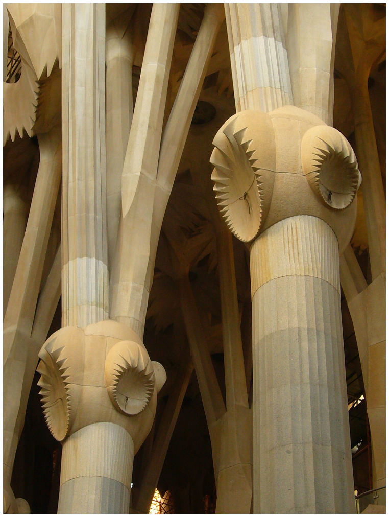
As seen in the figure, Gaudí imagined columns whose shape varies along the height. His goal was to mimic a stone forest and, for that, he modeled columns that branched from other columns (like tree branches), with the intersection between column brunches resembling tree knots. The variation of the columns’ shape is perfectly visible in some of these branches, in which the base is squared, but the top is nearly circular. In other cases, the column ends with a section in the shape of a star.
To model these columns, Gaudí spent two years elaborating a constructive scheme based on the intersection and union of helical shapes produced by the torsion of prisms [BarriosHernandez2006309]. In the simplest case, these prisms have a square section and suffer a torsion of sixteenths of a circle in both directions, i.e., \(2\pi/16=\pi/8\).
To generalize Gaudí’s approach, we will implement a function to deal with the general case of a prism with \(n\) sides, twisted at an arbitrary angle. For that, we will use the Khepri function surface_regular_polygon, which creates a regular polygon from the number of vertices \(n\), the polygon center \(P\), the distance \(r\) between the vertices and the point \(P\), and the angle \(\phi\) of the first vertex with the \(X\) axis.
To model the twisted prism, we will create a surface with the shape of the regular polygon and then we will extrude that surface to a height \(h\), while twisting it at an angle \(\Delta_\phi\) and applying a scale factor of \(e\):
twisted_prism(p, r, n, h, phi, dphi, f) =
sweep(line(p, p+vz(h)), surface_regular_polygon(n, u0(), r, phi), dphi, f)
To reproduce Gaudí’s approach, we intersect two of these prisms, both twisted at an angle of \(\pi/8\), but the first one in one direction and the second in the other direction. To be more realistic, we also apply a scale factor of 0.9, so that the column narrows as it goes up:
intersection(twisted_prism(xy(0, 0), 1, 4, 10, 0, pi/8, 0.9),
twisted_prism(xy(0, 0), 1, 4, 10, 0, pi/-8, 0.9))
The result is the leftmost column of this figure. The union of these prisms produces another of the shapes used by Gaudí, which is visible immediately to the right of the previous column:
union(twisted_prism(xy(5, 0), 1, 4, 10, 0, pi/8, 0.9),
twisted_prism(xy(5, 0), 1, 4, 10, 0, pi/-8, 0.9))
As done by Gaudí, we can complement the previous columns by doubling the number of prisms and halving the torsion angle:
intersection(twisted_prism(xy(10, 0), 1, 4, 10, 0, pi/16, 0.9),
twisted_prism(xy(10, 0), 1, 4, 10, 0, pi/-16, 0.9),
twisted_prism(xy(10, 0), 1, 4, 10, pi/4, pi/16, 0.9),
twisted_prism(xy(10, 0), 1, 4, 10, pi/4, pi/-16, 0.9))
union(twisted_prism(xy(15, 0), 1, 4, 10, 0, pi/16, 0.9),
twisted_prism(xy(15, 0), 1, 4, 10, 0, pi/-16, 0.9),
twisted_prism(xy(15, 0), 1, 4, 10, pi/4, pi/16, 0.9),
twisted_prism(xy(15, 0), 1, 4, 10, pi/4, pi/-16, 0.9))
The results are visible in the two columns on the right, in this figure.
Columns obtained by the intersection and union of twisted prisms with a square section.
7.8 Revolutions
A revolution is a surface or solid generated by rotating an object around an axis. A surface of revolution is a surface created by the rotation of a bi-dimensional curve around an axis. A solid of revolution is a solid generated by the rotation of a bi-dimensional region around an axis.
The revolution is a very simple process of creating surfaces and solids, and the Khepri’s function revolve serves exactly that purpose. The function receives the curve or region to revolve and, optionally, a point on the rotation axis (by omission, the origin), a vector parallel to the rotation axis (by omission, the vector with the \(Z\) axis direction), the initial angle of revolution (by omission, zero), and the angle increment for the revolution (by omission, \(2\pi\)). Naturally, if the increment is \(2\pi\) radians, we get a complete revolution.
7.8.1 Surfaces of Revolution
Using the revolve function, it is now easy to create surfaces or solids of revolution. For example, consider the spline presented in this figure, which was created from the following expression:
spline(xyz(0, 0, 2),
xyz(1, 0, -1),
xyz(2, 0, 1),
xyz(3, 0, -1),
xyz(4, 0, 0),
xyz(5, 0, -1))
A spline used as the base to build a surface of revolution.
Note that the spline is located on the \(XZ\) plane and, because of that, it can be used as the base to build a surface with the revolution axis in the \(Z\) axis. To better visualize the interior of the surface, we will consider an opening of \(\frac{2\cdot\pi}{4}\). The corresponding Julia expression is:
revolve(spline(xyz(0, 0, 2),
xyz(1, 0, -1),
xyz(2, 0, 1),
xyz(3, 0, -1),
xyz(4, 0, 0),
xyz(5, 0, -1)),
u0(),
vz(),
1/4*2*pi,
3/4*2*pi)
The result of evaluating the previous expression is represented in this figure.
A surface of revolution generated by the spline represented in this figure.
Surfaces of revolution are often used in architecture, namely, to design domes. The onion-shaped dome, for example, is a widely explored element in Russian and Mughal architectures, among others. The image in this figure shows the domes of Verkho Saviour Cathedral in Moscow, Russia.
Domes of the Verkho Saviour Cathedral in Moscow, Russia. Photograph by Amanda Graham.
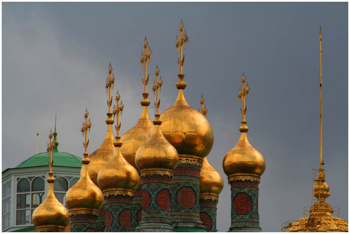
Onion-shaped domes possess an axial symmetry that allows them to be modeled as surfaces of revolution. For that, we will define a function called dome that, from an array of coordinates belonging to the dome’s profile, builds the surface of revolution that models the dome. To simplify, we will admit that the dome is closed at the top and that the top corresponds to the first element of the coordinates’ array. This simplification allows us to establish the surface revolution axis from the first element of the coordinates’ array:
dome(pts) =
revolve(spline(pts), pts[1])
To evaluate the function, we can get some coordinates from the profile of real domes and use them to invoke the function. That is precisely what we did in the following expressions:
dome([xyz(0, 0, 12),
xyz(0, 1, 8),
xyz(0, 6, 4),
xyz(0, 6, 2),
xyz(0, 5, 0)])
dome([xyz(15, 0, 9),
xyz(15, 3, 8),
xyz(15, 7, 5),
xyz(15, 8, 3),
xyz(15, 8, 2),
xyz(15, 7, 0)])
dome([xyz(30, 0, 13),
xyz(30, 1, 10),
xyz(30, 5, 7),
xyz(30, 5, 2),
xyz(30, 3, 0)])
which create, from left to right, the surfaces presented in this figure. Note that the dome function creates not only onion domes but also other types of domes.
Domes generated in Khepri.
7.8.1.1 Question 150
Consider the tube with a sinusoidal profile presented in the following image:
The tube was produced taking into account the geometrical parameters described in the following profile:
Define the function sinusoidal_tube that, from the previously illustrated parameters \(P\), \(r\), \(a\), \(omega\), \(lx\), and, finally, from the sinusoid’s phase \(phi\) and the separation between interpolation points \(\Delta_x\), generates the intended sinusoidal tube. For example, the tubes represented in the following image were generated by the evaluation of the following expressions:
sinusoidal_tube(xyz(-20, 80, 0), 20, 2.0, 0.5, 0, 60, 0.2)
sinusoidal_tube(xyz(0, 30, 0), 5, 0.2, 2.0, 0, 60, 0.1)
sinusoidal_tube(xyz(30, 0, 0), 10, 1.0, 1.0, pi/2, 60, 0.2)
7.8.1.2 Question 151
Consider an egg as a generalization of eggs of different proportions, as illustrated in the following image:
The egg’s section is sketched in the following image:
Define an egg function that creates a three-dimensional egg. The function should receive, only, the coordinates of point \(P\), the \(r_0\) and the \(r_1\) radii, and, finally, the height \(h\) of the egg.
7.8.2 Solids of Revolution
If, instead of using a curve to produce a surface of revolution, we use a region, the result will be a solid of revolution. As an example, imagine we use a trefoil to generate an arch. The image on the left of this figure shows the region used in the revolution, and this figure shows the created solid. For this example, we used the following expression:
A solid of revolution generated by the trefoil represented in this figure.
revolve(nfoil(xy(3, 0), 1, 3), u0(), vy(), 0, pi)
Through the combination of extrusions and revolutions, it is possible to produce very sophisticated models. Let us consider, for example, the modeling of an arcade whose columns and arches have sections in the shape of an nfoil. To model these shapes, it is necessary to know the position \(P\) of the center of the foil used to generate the column or the arch, the radius \(r_c\) of the columns and the number of foils \(n_f\) to use. It is also necessary to know the height \(h\) of the columns and the radius \(r_a\) of the arches. The following functions create the column and the arch:
nfoil_column(p, rc, nf, h) = extrusion(nfoil(p, rc, nf), h)
nfoil_arch(p, rc, ra, nf) = revolve(nfoil(p, rc, nf), p+vx(ra), vy(), 0, pi)
To build the arcade, the simplest way is to define a function that builds a column and an arch and that, recursively, builds the remaining arcades until it has no more arcades to build, the case at which it creates the last column that supports the last arch. The translation of this algorithm to Julia is:
nfoil_arcade(p, rc, nf, ra, h, n) =
if n == 0
nfoil_column(p, rc, nf, h)
else
union(nfoil_column(p, rc, nf, h),
nfoil_arch(p+vxyz(0, 0, h), rc, ra, nf),
nfoil_arcade(p+vxyz(2*ra, 0, 0), rc, nf, ra, h, n-1))
end
The image of this figure presents a perspective of a series of arcades generated by the following expressions:
nfoil_arcade(xy(0, 0), 1, 4, 5, 10, 5)
nfoil_arcade(xy(0, 10), 1, 6, 5, 10, 5)
nfoil_arcade(xy(0, 20), 1, 8, 5, 10, 5)
nfoil_arcade(xy(0, 30), 1, 10, 5, 10, 5)
nfoil_arcade(xy(0, 40), 1, 12, 5, 10, 5)
Arcades generated by the nfoil_arcade function. From the front to the back, the arcades have quatrefoil, sexfoil, octofoil, and so on, as section.
7.8.2.1 Question 152
We want to create a program capable of generating a barrel with the base located on the \(XY\) plane. Consider that the base of the barrel is closed but the top is open.
Create a function called profile_barrel that receives the point \(P\), both radii \(r_0\) and \(r_1\), the height \(h\), and the thickness \(t\), and returns the region that defines the profile of the barrel, as presented in the following image:
7.8.2.2 Question 153
Using the function profile_barrel, define the function barrel that, given the same parameters as the former one, creates a three-dimensional barrel. The function should have the following form:
barrel(p, r0, r1, h, t) = ___
As an example, consider the following image that was generated by the evaluation of the following expressions:
barrel(xyz(0, 0, 0), 1, 1.3, 4, 0.1)
barrel(xyz(4, 0, 0), 1, 1.5, 3, 0.3)
barrel(xyz(8, 0, 0), 1, 0.8, 5, 0.1)
7.8.2.3 Question 154
The barrel function created in the previous exercise is unable to generate the traditional wooden barrels that are built from wooden staves put together next to each other. The following image shows a few examples of these wooden staves, with different dimensions and placements:
Define the function barrel_stave that, besides the same parameters that define a barrel, also receives an initial rotation angle \(\alpha\), which defines where the stave begins, and an angle increment \(\Delta_\alpha\), which corresponds to the angular amplitude of the stave, and builds the three-dimensional section of the barrel corresponding to the stave in question.
7.8.2.4 Question 155
Define a function called barrel_staves that receives as parameters the point \(P\), the radii \(r_0\) and \(r_1\), the height \(h\), the thickness \(t\), the number of staves \(n\), and the angular spacing \(s\) between staves, and creates a three-dimensional barrel with that number of staves. The following image shows some examples of these barrels, which were created by the evaluation of the following expressions:
barrel_staves(xyz(0, 0, 0), 1, 1.3, 4, 0.1, 10, 0.05)
barrel_staves(xyz(4, 0, 0), 1, 1.3, 4, 0.1, 4, 0.5)
barrel_staves(xyz(8, 0, 0), 1, 1.3, 4, 0.1, 20, 0.01)
7.9 Sections Interpolation
Section interpolation, also known as shape morphing, allows the creation of a three-dimensional object through the interpolation of planar sections. In Khepri, this interpolation is implemented by the loft and the loft_ruled functions. These functions operate from an ordered array of planar sections (that might be curves or regions), which can be optionally complemented with guidelines to minimize possible mistakes in the interpolation process. The use of guidelines is particularly important in the case of planar sections with rectilinear parts.
In the next sections, we will analyze separately each of these forms of interpolation.
7.9.1 Interpolation without Guidelines
There are two fundamental ways of doing shape interpolation without guidelines: by generating a ruled surface (i.e., surfaces generated by a movement of a line segment) between each planar section, or by generating a smooth surface (i.e., without sudden slope shifts) that comes closer to several planar sections. The interpolation by ruled surfaces is implemented by the loft_ruled function, while the interpolation by smooth surfaces is done with the loft function.
To compare the effects of these two functions, consider the following expression that creates a ruled surface interpolation from three circles, represented on the left of this figure:
let circ0 = surface_circle(xyz(0, 0, 0), 4),
circ1 = surface_circle(xyz(0, 0, 2), 2),
circ2 = surface_circle(xyz(0, 0, 4), 3)
loft_ruled([circ0, circ1, circ2])
end
In the same this figure, on the right, we can find a smooth surface interpolation of the same three circles, generated by the following expressions:
let circ0 = surface_circle(xyz(0, 9, 0), 4),
circ1 = surface_circle(xyz(0, 9, 2), 2),
circ2 = surface_circle(xyz(0, 9, 4), 3)
loft([circ0, circ1, circ2])
end
Surface interpolation of three circles: on the left, with a ruled surface interpolation, and on the right, with a smooth surface interpolation.
7.9.2 Interpolation with Guidelines
It is relatively obvious that there is an unlimited number of different surfaces that interpolate two given sections. Unfortunately, not all of them match the desired outcome, especially when it is necessary to produce an interpolation between two very different sections.
Different interpolations are produced depending not only on the CAD application that is being used but also on the version of that application.
loft(
[surface_regular_polygon(
6, xyz(0, 0, 0), 1.0, 0),
surface_regular_polygon(
3, xyz(0, 0, 5), 0.5, pi/6)])
Note that, on the left side of this figure, one of the sides of the triangle is directly mapped into one of the sides of the hexagon, thus forcing the interpolation to distort the remaining two sides of the triangle to map the remaining five sides of the hexagon.
Fortunately, the loft function offers other ways of doing interpolation that minimize the possibility of errors. This function receives not only the array of sections to interpolate, but also an array of curves that guide the interpolation process. Using this function, we can reproduce the interpolation on the right of this figure by establishing guidelines between the relevant vertices of each polygon. These guidelines will force Khepri to generate an interpolation that integrates these lines on the generated surface, and thus controlling the pairing of points between the sections to interpolate. To that end, we will generate three vertices of the hexagon that, together with the three vertices of the triangle, allow the creation of the guidelines.
Since we need to build the guidelines from the polygons’ vertices, we will start by defining a function that, with two arrays of points, creates an array of lines that use one point of each array at a time:
guides(p0s, p1s) =
if p0s == []
[]
else
[line(p0s[1], p1s[1]),
guides(p0s[2:end],
p1s[2:end])...]
end
Next, we generate three non-consecutive vertices of the hexagon that, together with those of the triangle, allow the creation of the guidelines:
loft(
[surface_regular_polygon(
6, xyz(3, 0, 0), 1.0, 0),
surface_regular_polygon(
3, xyz(3, 0, 5), 0.5, pi/6)],
guides(
regular_polygon_vertices(
3, xyz(3, 0, 0), 1.0, 0),
regular_polygon_vertices(
3, xyz(3, 0, 5), 0.5, pi/6)))
The evaluation of the previous expression allows Khepri to produce a more uniform interpolation between the hexagon and the triangle, as can be seen on the right side of this figure.
Top view of an interpolation between a hexagonal section and a triangular section. On the left, the interpolation was performed without guidelines. On the right, the interpolation was performed with guidelines, associating three non-consecutive of the hexagon to the three vertices of the triangle.
7.9.2.1 Question 156
Consider the interpolation between two random closed curves positioned on different heights, as presented in the following figure:
Each curve is a spline produced with points generated by the random_circle_points function defined in the exercise of Question 103. Write an expression capable of generating a solid similar to the ones presented in the previous image.
8 Transformations
8.1 Introduction
All the objects created so far had a definitive nature: the parameters used to build them univocally define the shape of those objects. All we can do is invoke the functions that create these objects with different parameters to build different objects.
Although that way of creating objects is powerful enough, there are alternatives potentially more practical that are based in the modification of previously created objects. That modification is performed through the operations of translation, rotation, reflection and scale.
It is important to note that these operations do not create new objects; they only affect objects to which they are applied. For example, after applying a translation to an object, this object simply changes its position.
However, sometimes we want to apply transformations that produce new objects as a result. For example, we might want to produce a translation of an object, but leaving the original object in its original place. One way of doing this is to apply the translation operation, not to the original object, but to a copy of it. For this purpose, Khepri provides the copy_shape operation that receives an object as an argument and returns a copy of that object, situated in the exact same place as the original. Naturally, in the CAD tool, two equal overlapping objects will appear. Typically, the copied object will subsequently be transformed, for example, by moving it to another location.
In the next sections, we will discuss the transformation operations available in Khepri.
8.2 Translation
The translation operation moves an object by adding a vector to all its points, causing all these points to move a certain distance in a determined direction. The vector components indicate what is the displacement in relation to each coordinate axis.
To perform the translation operation, Khepri provides the move operation, which receives one object and one displacement vector. As an example, we have:
move(sphere(), vxyz(1, 2, 3))
Note that the function returns the object that suffered the translation to allow its combination with other operations.
For the previous example, it is simpler to immediately specify the sphere’s center by writing:
sphere(xyz(1, 2, 3))
However, in more complex cases, it can be advantageous to consider an object created at the origin and later translated to the desired position. Let us consider, for example, a papal cross, defined by the union of three horizontal cylinders of progressively decreasing length placed along a vertical cylinder, as can be seen in this figure.
A papal cross.
All cylinders have the same radius, and their length and position are defined according to that radius. The vertical cylinder of the papal cross has a length equal to \(20\) radii, while the horizontal cylinders have lengths equal to \(14\), \(10\) and \(6\) radii. Their axes are positioned at a height equal to \(9\), \(13\) and \(17\) radii. These proportions are implemented by the following function, which receives a reference point \(P\) and a radius \(r\):
papal_cross(p, r) =
union(cylinder(p, r, p+vz(20*r)),
cylinder(p+vxz(-7*r, 9*r), r, p+vxz(7*r, 9*r)),
cylinder(p+vxz(-5*r, 13*r), r, p+vxz(5*r, 13*r)),
cylinder(p+vxz(-3*r, 17*r), r, p+vxz(3*r, 17*r)))
However, if we assume that the cross is initially positioned at the origin, we can slightly simplify the previous definition:
papal_cross(r) =
union(cylinder(u0(), r, z(20*r)),
cylinder(xz(-7*r, 9*r), r, xz(7*r, 9*r)),
cylinder(xz(-5*r, 13*r), r, xz(5*r, 13*r)),
cylinder(xz(-3*r, 17*r), r, xz(3*r, 17*r)))
Naturally, if we want to place the cross at a specific position, for example, \((1,2)\), we should write:
move(papal_cross(1), vxy(1, 2))
8.3 Scale
The scale transformation increases or decreases the dimension of an entity without changing its shape. This operation is also called homothety. Although it is conceivable to have a scale operation that modifies each dimension independently, it is more usual to employ a uniform scale that modifies simultaneously the three dimensions, affecting them with the same factor. If the factor is bigger than one, the size increases. If the fact is smaller than one, the size decreases.
In the case of Khepri, only a uniform scale operation is provided, given by the scale function.
The scale transformation, besides changing the object’s dimension, can also change its position. If that is not the intended case, we can previously apply a translation to center the object in the origin, then apply the scale operation and finally apply the inverse translation to return the object to its original position.
By using the scale operation, it is possible to further simplify the previous definition of the papal cross. In fact, because the cross dimension depends only on the radius, we can arbitrate a unit radius which we can later change through a scale operation. That way, we can write:
papal_cross() =
union(cylinder(u0(), 1, 20),
cylinder(xz(-7, 9), 1, xz(7, 9)),
cylinder(xz(-5, 13), 1, xz(5, 13)),
cylinder(xz(-3, 17), 1, xz(3, 17)))
If we want to build a papal cross with a determined radius \(r\), for example, \(r=3\), we only need to write:
scale(papal_cross(), 3)
8.4 Rotation
In the rotation operation, all the object’s points are moved in a circular motion in turn of a point (two dimensions) or an axis (three dimensions). In the general case of a three dimensional rotation, it is usual to decompose it into three successive rotations around the coordinate axes. These rotations around the \(X\), \(Y\), and \(Z\) axes are called main rotations. In Khepri, each of these rotations is performed by the rotate function that receives, as arguments, the object on which the rotation is applied, the rotation angle, and the rotation axis defined by a position and a vector. By omission, the rotation will be performed in relation to the \(Z\) axis.
This figure illustrates some combinations of translations, scales and rotations, generated by the following program:
papal_cross()
move(papal_cross(), vx(20))
move(scale(papal_cross(), 1.25), vx(40))
move(rotate(scale(papal_cross(), 1.5), pi/4), vx(60))
move(rotate(scale(papal_cross(), 1.75), pi/4, u0(), vx()), vx(80))
A papal cross of unit radius placed at the origin (on the left), transformed by the following operations (from left to right): translation, scale with translation, scale with rotation and translation and, finally, scale with rotation around the \(X\) axis and translation.
8.5 Reflection
In addition to the translation, scale and rotation operations, Khepri also implements the reflection operation, by providing the function mirror. This function receives, as arguments, the object to reflect, and a reflection plane described by a point contained in the plane and a normal vector to the plane. By omission, the reflection plane is the \(XY\) plane.
As an example, let us consider the hourglass shown in this figure that has as parameters the base center point, the base radius, the neck radius, and the height.
An hourglass.
It is not difficult to conceive this shape as the union of two cone frustums:
hourglass(p, rb, rn, h) =
union(cone_frustum(p, rb, p+vz(h/2), rn),
cone_frustum(p+vz(h/2), rn, p+vz(h), rb))
However, it is possible to simplify the previous definition by using the mirror operation:
hourglass(p, rb, rn, h) = mirror(cone_frustum(p, rb, p+vz(h/2), rn), p+vz(h/2))
In the following section, we will see an example where these operations are applied in the modeling of one of the most famous buildings in the world.
8.6 The Sydney Opera House
The Sydney Opera House resulted from an international competition launched in 1955 for the design of a building dedicated to performing arts. The winner, announced in 1957, was the project of Jørn Utzon, a Danish architect little known until then. His project, even though not fully satisfying the competition requirements, was selected by one of the jury members - the famous architect Eero Saarinen - that foreseen it as a landmark project. The proposal consisted in a set of shell-shaped roof structures, capable of accommodating various performance venues. The result of this final proposal is represented in this figure.
The Sydney Opera House. Photograph by Brent Pearson.
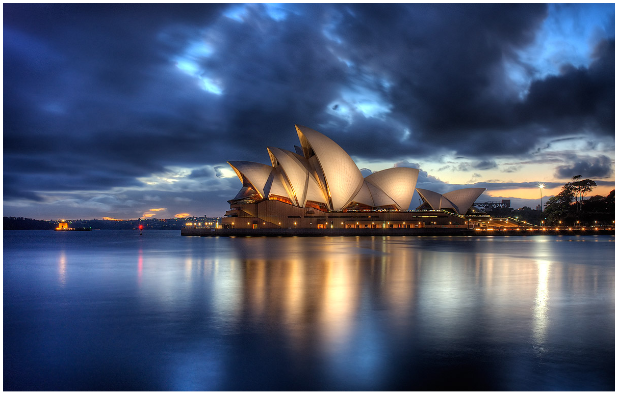
Clearly innovative, the Utzon’s design was too advanced for the design and construction technologies of the time and was by many considered impossible. In the three years that followed the start of the construction in 1959, Utzon, along with the structural engineering team of the Ove Arup company, tried to find a mathematical formulation for his hand-drawn shells. A variety of different approaches were experimented, including parabolic, circular and elliptical shapes, but all of the solutions had, besides enormous technical difficulties, very high costs that were completely incompatible with the approved budget.
In the summer of 1961, Utzon was on the brink of despair and decided to dismantle the shells’ Perspex model. However, when stacking the shells for storage, he found that they fit almost perfectly inside each other, which would only be possible if the different shells had the same curvature at all its points. Incidentally, the surface that has the same curvature at all its points is the sphere, which led Utzon to think that maybe it would be possible to shape his shells as cut triangles from a sphere’s surface. Although this design was not exactly identical to the original drawings, it had the advantage of being calculable in computers and, more importantly, of allowing a more economic construction. Utzon’s idea is explained in a bronze model placed next to the building of the Opera House, as can be seen in this figure.
Bronze plaque explaining Utzon’s idea for modeling the shells. Photograph by Matt Prebble.
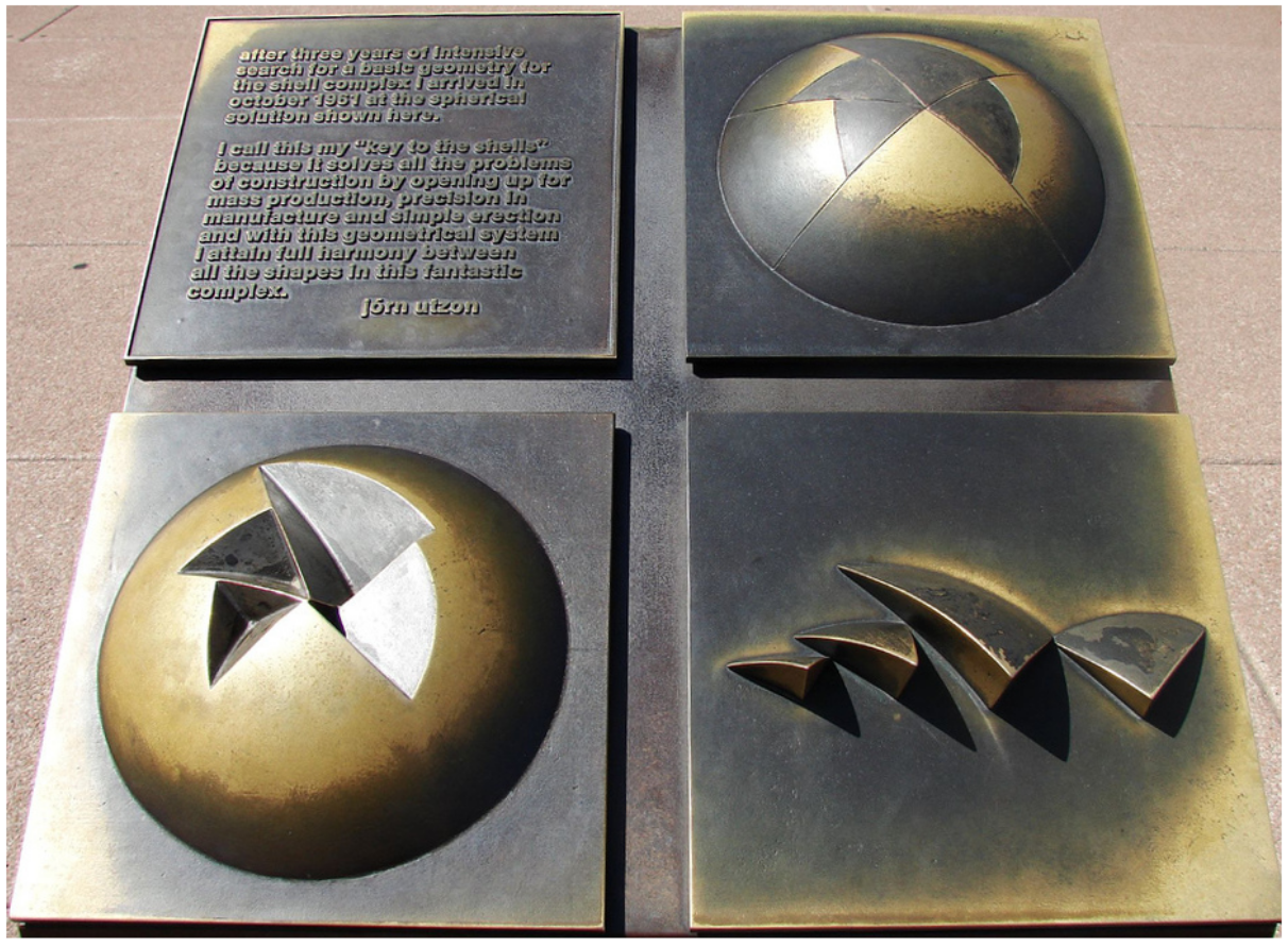
Despite Utzon’s personal drama, this story turned out to have a happy ending: thirty years later, the Australian government remodeled the Sydney Opera House to reunite the masterpiece with its architect and got Utzon, who never got to see his work finished, to be engaged with the refurbishment, aiming to rearticulate the exterior with the interior.
In this section, we will model the shells of the Sydney Opera House following exactly the same solution proposed by Utzon. All the building shells will be modeled by spherical triangles obtained by three cuts in a sphere. This figure shows two spheres of equal radius from which we cut two triangles, in order to get two of the half-shells that constitute the Sydney Opera House.
Two of the half-shells that constitute the Sydney Opera House, and the spheres from where they were obtained by a succession of cuts.
To define the section planes that will cut the triangles we can consider that the building will be aligned in a direction parallel to the \(Y\) axis, so the shell’s symmetry axis will correspond to a section plane whose normal is the \(X\) axis, as can be seen in this figure. The two remaining section planes will have normals determined so as to approximate, as rigorously as we can, the volumes imagined by Utzon. As is also visible in this figure, the half-shells are extracted from spheres with equal radius but centered at different positions. Thus, to model these half-shells we are going to define a function that, from the center \(P\) of the sphere of radius \(r\) and the normals \(n_1\) and \(n_2\) of the section planes, produces a spherical shell with thickness \(t\) and with the desired shape.
Top view of two of the half-shells that constitute the Sydney Opera House, and the spheres from which they were obtained by a succession of cuts.
half_shell(p, r, t, n1, n2) =
move(slice(slice(slice(subtraction(sphere(u0(), r),
sphere(u0(), r-t)),
u0(),
n2),
u0(),
n1),
x(-p.x),
-vx()),
p-u0())
As an example, this figure shows a half-shell generated by evaluating the following expression:
half_shell(xyz(-45, 0, 0), 75, 2, vsph(1, 2.0, 4.6), vsph(1, 1.9, 2.6))
A half-shell of the Sydney Opera House.
To produce a complete shell, we only have to apply a reflection to the half-shell by the vertical section plane:
shell(p, r, t, n1, n2) = mirror(half_shell(p, r, t, n1, n2), u0(), -vx())
This figure shows the shell generated by evaluating the following expression:
shell(xyz(-45, 0, 0), 75, 2, vsph(1, 2.0, 4.6), vsph(1, 1.9, 2.6))
A Sydney Opera House shell.
To define a row of shells of the Opera House we will use values that approximate the produced shells with Utzon’s original drawing:
row_shells() =
union([shell(xyz(-45.01, 0.0, 0.0), 75, 2,
vsph(1, 1.9701, 4.5693), vsph(1, 1.9125, 2.5569)),
shell(xyz(-38.92, -13.41, -18.85), 75, 2,
vsph(1, 1.9314, 4.5902), vsph(1, 1.7495, 1.9984)),
shell(xyz(-38.69, -23.04, -29.89), 75, 2,
vsph(1, 1.9324, 4.3982), vsph(1, 1.5177, 1.9373)),
shell(xyz(-58.16, 81.63, -14.32), 75, 2,
vsph(1, 1.6921, 3.9828), vsph(1, 1.4156, 1.9618)),
shell(xyz(-32.0, 73.0, -5.0), 75, 2,
vsph(1, 0.91, 4.1888), vsph(1, 0.8727, 1.3439)),
shell(xyz(-33.0, 44.0, -20.0), 75, 2,
vsph(1, 1.27, 4.1015), vsph(1, 1.1554, 1.2217))])
Invoking this function will produce the row of shells presented in this figure.
A row of shells of the Sydney Opera House.
In order to facilitate the positioning of the building, we will include a rotation around the \(Z\) axis, a scaling, and a final translation applied to each row of shells. Since the building has two rows of shells, we will call this function half_opera_sydney:
half_opera_sydney(rot_z, sca, trans_x) =
move(scale(rotate(row_shells(), rot_z), sca),
vx(trans_x))
Finally, we can model the entire Opera House by making a row of shells at a scale of \(1.0\) and a second row of shells as a reduced, rotated and shifted version of the first. The scale used by Utzon was \(0.8\), and the rotation angles and the translations that we are going to use are those that allow us a higher resemblance to the actual building:
opera_sydney() =
begin
half_opera_sydney(0.1964, 1.0, 43)
half_opera_sydney(-0.1964, 0.8, -15)
end
The final result of modeling the shells of the Sydney Opera House is shown in this figure.
The complete model of shells of the Sydney Opera House.
8.6.1 Exercises 36
8.6.1.1 Question 157
Define a function that creates a link of a chain, such as the one shown on the left of the following image.
To simplify the modeling process, consider the link as decomposable into fourths of a link, as shown on the right of the previous image. This way, it will be enough to define a function that creates a fourth of a link (composed by a quarter of a torus and a cylinder), and then apply a double reflection in the \(X\) and \(Y\) axes to compose the complete link.
The function should receive, as parameters, the radius \(r_l\) of the link, the radius \(r_i\) of the wire, and the length \(l\) between the semi-circles, such as shown in the following scheme.
8.6.1.2 Question 158
Define a function capable of creating chains such as those presented below:
8.6.1.3 Question 159
Define a function to create closed chains such as the one presented below:
Note that the links suffer successive rotations around the \(X\) axis.
9 Higher-Order Functions
9.1 Introduction
We have been demonstrating how the Julia language can enable us, through the definition of appropriate functions, to create the architectural forms that we have in mind. One of the advantages of the definition of these functions is that many of these architectural forms become parametrized, allowing us to easily try variations until we reach the numerical values of the parameters that satisfy us.
Despite the "infinite" variability that the parameters allow us, there will always be limits to what we can do with only numerical parameters, and for us to have a superlative degree of variability, we will also have to vary the actual functions.
In this section we will discuss higher-order functions. A higher-order function is a function that receives functions as arguments or a function that returns functions as result. Apart from this feature a higher-order function is no different from any other function.
9.2 Curvy Facades
To motivate the discussion let us consider a simple problem: we intend
on idealizing a building where three of the sides are planar and the
fourth —
As seen in section Extrusions, a sinusoid is determined by a set of parameters, such as the amplitude \(a\), the number of cycles per length unit \(omega\) and the phase \(phi\) of the curve in relation to the \(y\) axis. With these parameters the sinusoid curve equation has the form: \(y(x) = a \sin(\omega x + \phi)\)
To calculate the points of a sinusoid we can use the function sinusoid_points that computes a list of coordinates \((x,y)\) corresponding to the evolution of a sinusoid between the limits of a range \([x_0, x_1]\), with an increment \(\Delta_x\);
sinusoid_points(p, a, omega, phi, x0, x1, dx) =
if x0 > x1
[]
else
[p+vxy(x0, sinusoid(a, omega, phi, x0)),
sinusoid_points(p, a, omega, phi, x0+dx, x1, dx)...]
end
The previous function generates a list with the point of the facade. In order to model the rest of the building we need to join these points to form a curve and we need to join the three rectilinear sides in order to form a region that corresponds to the building floor plan. For this, we will connect the points with a spline and form a region between it and the lines that delimit the other three sides of the building. The length \(l_x\) of the building will be given by the horizontal distance between the two ends of the curve of the facade. The width \(l_y\) and height \(l_z\) will have to be parameters. Thus, we have:
building(points, ly, lz) =
let p0 = points[1],
p1 = points[end],
lx = p1.x-p0.x
extrusion(surface_from(spline(points),
line(p0, p0+vxy(0, ly), p0+vxy(lx, ly), p1)),
lz)
end
To visualize the capabilities of the previous function we can build several buildings using different values for the sinusoid’s parameters. In the following expressions we considered two rows of buildings, all with \(15\) meters long, \(10\) meters wide and \(20\) or \(30\) meters tall, depending on the row. This figure shows these buildings for different values of the parameters a, omega and fi:
Urbanization of buildings of which the facade corresponds to sinusoidal walls with different parameters.
building(sinusoid_points(xy(0, 0), 0.75, 0.5, 0, 0, 15, 0.4), 10, 20)
building(sinusoid_points(xy(25, 0), 0.55, 1.0, 0, 0, 15, 0.2), 10, 20)
building(sinusoid_points(xy(50, 0), 0.25, 2.0, 0, 0, 15, 0.1), 10, 20)
building(sinusoid_points(xy(0, 20), 0.95, 1.5, 0, 1, 15, 0.4), 10, 30)
building(sinusoid_points(xy(25, 20), 0.85, 0.2, 0, 0, 15, 0.2), 10, 30)
building(sinusoid_points(xy(50, 20), 0.35, 1.0, 0, 1, 15, 0.1), 10, 30)
Unfortunately, although the sinusoid_points function is very useful for modeling a multitude of different buildings with a sinusoidal facade, it is totally useless to model buildings of which the facade follows a parabola or a logarithm or an exponential or, in fact, any other curve which is not reducible to a sinusoid. In fact, although the adjustment of the parameters allows us infinite variability of the modeled building, even then it will always be a particular case of a sinusoidal facade.
Naturally nothing prevents us from defining other functions for modeling different facades. Let us imagine, for example, that we want a facade with the curvature of a parabola. The parabola with vertex at \((x_v,y_v)\) and focus point at \((x_v,y_v+d)\), with \(d\) being the distance from the vertex to the focus point, is defined by the following equation:
\[(x - x_v)^2 = 4d(y - y_v)\]
that is
\[y=\frac{(x - x_v)^2}{4d}+y_v\]
In Julia, this function is defined as:
parabola(xv, yv, d, x) = (x-xv)^2/(4*d)+yv
In order to generate the parabola’s points we have, as usual, to iterate over a range \([x_0, x_1]\) with a certain increment \(Delta_x\):
parabola_points(p, xv, yv, d, x0, x1, dx) =
if x0 > x1
[]
else
[p+vxy(x0, parabola(xv, yv, d, x0)),
parabola_points(p, xv, yv, d, x0+dx, x1, dx)...]
end
The following expressions test this function with different values of the various parameters:
building(parabola_points(xy(0, 0), 10, 0, 5, 0, 15, 0.5), 10, 20)
building(parabola_points(xy(25, 0), 5, 0, 3, 0, 15, 0.2), 10, 20)
building(parabola_points(xy(50, 0), 7, 1, -2, 0, 15, 0.1), 10, 20)
building(parabola_points(xy(0, 20), 8, 0, 2, 0, 15, 0.4), 10, 30)
building(parabola_points(xy(25, 20), 6, -2, 3, 0, 15, 0.2), 10, 30)
building(parabola_points(xy(50, 20), 5, 0, 6, 0, 15, 0.1), 10, 30)
generating the "urbanization" represented in this figure.
Urbanization of buildings of which the facade corresponds to paraboloidal walls with different parameters.
Once more, the parametrization of the function
parabola_points allows us to generate an infinity of buildings
of which the facade has the curvature of a parabola, but they will always be
different buildings from those that we can create with the sinusoid_points
function. Although the modeling process used is absolutely
identical in both cases, the applied base functions—
Clearly, if we now want to create buildings with a curved facade determined by a function \(f(x)\) that is neither a sinusoid nor a parabola, we can not employ the previous functions. First, we will need to define the function f that implements that curve and, second, we will need to define the f_points function that generates the points of f in an interval. This second part seems overly repetitive and, indeed, it is. We simply have to observe the sinusoid_points and parabola_points functions to conclude that they are very similar to each other. Logically, the same will happen with the new f_points function.
This repetition leads us to consider the possibility of abstracting the processes in question so that we are not obliged to repeat definitions that only vary in small details. For this, we can start by comparing the definitions of the functions and understand where the differences are.
It now becomes absolutely clear that the only difference between the two functions lies in an invocation they make, which is sinusoid in one case and parabola in the other.
Now, when two functions differ only in a name they use internally, it is always possible to define a third function that generalizes them, simply transforming that name into an additional parameter.
Suppose then that we make the following definition, where f is this additional parameter:
function_points(p, f, alpha, beta, gamma, x0, x1, dx) =
if x0 > x1
[]
else
[p+vxy(x0, f(alpha, beta, gamma, x0)),
function_points(p, f, alpha, beta, gamma, x0+dx, x1, dx)...]
end
The innovative look of the function_points function lies in the fact that it receives a function as an argument, a function which will be associated to the parameter f. When, in the body of the function_points function, a call is made of the f function, we are, actually, calling the function that has been passed as argument to the f parameter.
Thus, the expression
sinusoid_points(p, a, omega, phi, 0, lx, dx)
is absolutely identical to
function_points(p, sinusoid, a, omega, phi, 0, lx, dx)
Similarly, the expression
parabola_points(p, xv, yv, d, 0, lx, dx)
is absolutely identical to
function_points(p, parabola, xv, yv, d, 0, lx, dx)
More important than the fact that we can dismiss the sinusoid_points and parabola_points functions is the fact that, now, we can model buildings of which the facades follow any other curve we want. For example, the function that describes the damped oscillatory motion has the definition:
\[y=ae^{-bx}\sin(cx)\]
or, in Julia:
damped_oscillatory(a, b, c, x) = a*exp(-(b*x))*sin(c*x)
Using the function_points function, it is now trivial to define a building of which the facade follows the curve of the damped oscillatory motion. For example, the following expression
building(function_points(xy(0, 0), damped_oscillatory, -5, 0.1, 1, 0, 40, 0.4),
10,
20)
produces, as a result of its evaluation, the building presented in this figure.
A building with a facade that follows the curve of the damped oscillatory motion.
9.3 Higher-Order Functions
The function_points function is an example of a class of functions which we call higher-order. A higher-order function is a function that receives other functions as arguments or returns other functions as result. In the case of the function_points function it receives a function of a parameter that will be called in successive interval points, producing the list of the found coordinates.
Higher-order functions are important tools for abstraction. They allow the abstraction of computations in which there is a part of the computation that is common and one (or more parts) that vary from case to case. Using a higher-order function, we only implement the part of the computation that is common, leaving the variable parts of the computation to be implemented as functions that will be passed in the parameters of the higher-order function.
The concept of higher-order function exists for a long time in mathematics, although rarely explicitly mentioned. Let us consider, for example, a function which sums the squares of all integers between \(a\) and \(b\), \(\sum_{i=a}^{b}i^2\):
square_sum(a, b) =
if a > b
0
else
a^2+square_sum(a+1, b)
end
> square_sum(1, 4)
30
Let us now consider another function that sums the square roots of all the integers between \(a\) and \(b\), \(\sum_{i=a}^{b}\sqrt{i}\):
square_roots_sum(a, b) =
if a > b
0
else
sqrt(a)+square_roots_sum(a+1, b)
end
> square_roots_sum(1, 4)
6.146264369941973
The mere observation of the functions’ definition shows that they have a common structure characterized by the following definition:
sum_???(a, b) =
if a > b
0
else
???(a)+sum_???(a+1, b)
end
Now, this definition is no more than a sum of a mathematical expression between two limits, i.e., a summation \(\sum_{i=a}^{b}f(i)\). The summation is a mathematical abstraction for a sum of numbers described by a mathematical expression relative to the summation index which ranges from the lower to the upper limit. The mathematical expression is, therefore, a function of the summation index.
The symbol ??? represents the mathematical expression to perform inside the sum and that we will simply transform into a parameter, by writing:
summation(f, a, b) =
if a > b
0
else
f(a)+summation(f, a+1, b)
end
We can now trivially evaluate different summations:
>
summation(sqr, 1, 4)
30
>
summation(sqrt, 1, 4)
6.14626
Because it accepts a function as an argument, the sum is a
higher-order function. The derivative of a function is another
example. The derivative \(f'\) of a function \(f\) is a function that
receives another function \(f\) as argument and returns another
function—
Generally, higher-order functions show up because there are two or more functions with a similar structure. In fact, the repetition of a pattern along two or more functions is a strong indicator of the need for a higher-order function.
9.4 Anonymous Functions
The possibility of using higher-order functions opens up a huge range of new applications. For example, if we want to calculate the summations \[\sum_{i=1}^{10}i^2+3i\] \[\sum_{i=1}^{100}i^3+2i^2+5i\] we need not do more than to define the functions \(f_1(x)=x^2+3x\) and \(f_2(x)=x^3+2x^2+5x\) and use them as argument of the summation function:
f1(x) = x*x+3*x
f2(x) = x*x*x+2*x*x+5*x
> summation(f1, 1, 10)
550
> summation(f2, 1, 100)
26204450
As can be seen, we can now easily calculate summations of different functions. However, there is a negative aspect to note: if, for each summation we intend on calculating, we have to define the function in question, we will "pollute" our Julia environment with countless definitions of functions of which their utility will be, at most, to serve as argument to calculate the corresponding summation. Since each function must be associated with a name, we will also have to come up with names for all of them, which could be difficult, particularly, when we know that these functions are useful for nothing else. In the last two examples this problem was already visible: the names f1 and f2 only reveal the difficulty in finding more expressive names.
In order to solve this problem, we should examine in greater detail the concept of defining a function. So far we have said that, for defining a function, we have to use a combination that begins with the word define, followed by a list in which the first element is the name of the function to define and of which the remaining elements are the function’s parameters, followed by the function’s body. For example, for the function \(x^2=x\times x\), we write:
sqr(x) = x*x
We have seen that after the previous definition, the sqr symbol becomes associated with a function:
> sqr
sqr (generic function with 1 method)
However, we saw in section Global Variables that in order to define constants we should use the define operator in a combination that includes the name we want to define followed by the expression that we intend to associate with that name. For example:
phi = (1+sqrt(5))/2
We also saw that after the previous definition, the fi symbol becomes associated with a value:
> fi
ERROR: UndefVarError: fi not defined
The name lambda expression derives from the origins of the mathematical concept of anonymous function: the \(\lambda\) calculus, a mathematical model for computable functions, i.e., functions whose invocation can be evaluated mechanically.
In Julia, lambda expressions have the syntax (param1, param2, ...) -> expression. When the function has only one parameter, the syntax can be simplified, becoming param -> expression.
Notice the following:
> x -> x*x
#17 (generic function with 1 method)
> my_sqr = x -> x*x
#19 (generic function with 1 method)
> my_sqr(3)
9
As you can seen, the evaluation of the lambda expression returns something of which the external representation indicates that a procedure was created. When we associate the anonymous function with a name, that name becomes the designation of the function, and can be used as if it had been originally defined as a function. This equivalence is easily tested with the redefinition of functions that, now, can be defined as the creation of an association between a name and an anonymous function. The previous example demonstrated this possibility for the my_sqr function but it exists for any other function. For example, the function that calculates the area of a circle can be defined by either:
circle_area(radius) = pi*radius^2
or by:
circle_area = radius -> pi*radius^2
Although from the syntactic point of view, the form f(___) = ___ is equivalent to f = ___ -> ___, there is a semantic difference with important implications: the first form does not evaluate any of its arguments, whereas the latter form evaluates its second argument. This allows the second form to define functions with more sophisticated forms.
The use of anonymous functions has yet another advantage that becomes evident when we analyze the function_points function:
function_points(p, f, alpha, beta, gamma, x0, x1, dx) =
if x0 > x1
[]
else
[p+vxy(x0, f(alpha, beta, gamma, x0)),
function_points(p, f, alpha, beta, gamma, x0+dx, x1, dx)...]
end
As we have seen, in order to generate a list of points of, for example, a sinusoid, we can invoke this function the following way:
function_points(xy(0, 0), sinusoid, 0.75, 0.5, 0, 0, 15, 0.4)
Note that, for having been defined as a generalization of the functions sinusoid_points and parabola_points, the function function_points, in addition to having introduced the f function as a parameter, it also generalized the a, omega and fi parameters of the function sinusoid_points and xv, yv and d of the function parabola_points, calling them, respectively, alpha, beta and gamma. It so happens that these parameters never change during the recursive calls performed by the function_points function. In fact, the function passes these parameters from recursive call to recursive call only because they are necessary for the invocation of the f function. Let us now imagine that, instead of passing these parameters, they were associated to the f function itself that we had just passed. In this case, we could rewrite the function_points function in the following form:
function_points(p, f, x0, x1, dx) =
if x0 > x1
[]
else
[p+vxy(x0, f(x0)), function_points(p, f, x0+dx, x1, dx)...]
end
With this new definition, the previous call would have to be rewritten as:
function_points(xy(0, 0), x -> sinusoid(0.75, 0.5, 0, x), 0, 15, 0.4)
Although it may not seem to be a substantial gain, rewriting the function function_points has a considerable advantage: it allows the use of any base functions, regardless of the number of parameters it has: if they have only one parameter, they can be used directly, otherwise we can "wrap" them with an anonymous function of one parameter only that invokes the desired function with all the required arguments. This makes the function function_points even more generic, as it is visible in following examples:
> spline(function_points(xy(0, 6), sin, 0, 4*pi, 0.2))
Spline(...)
> spline(function_points(xy(0, 3), x -> -(x/10)^3, 0, 4*pi, 0.5))
Spline(...)
> spline(function_points(xy(0, 0), x -> damped_oscillatory(1.5, 0.4, 4, x), 0, 4*pi, 0.05))
Spline(...)
which create the curves shown in this figure.
Curve generated by the function function_points. From top to bottom, we have a sinusoid, an inverted exponential and a damped sinusoid.
Even though the generalization of higher-order functions allows these to be used in a wide variety of situations, sometimes, it is preferable to encapsulate a particular use in a function more easily recognizable. For example, if a program is systematically computing points of a sinusoid, then it is likely that this program becomes more readable if in fact the sinusoid_points function exists. But even in this case, the order functions will allow this function to be defined in a simpler way. That way, instead of having to write the usual recursive definition:
sinusoid_points(p, a, omega, phi, x0, x1, dx) =
if x0 > x1
[]
else
[p+vxy(x0, sinusoid(a, omega, phi, x0)),
sinusoid_points(p, a, omega, phi, x0+dx, x1, dx)...]
end
we can now write:
sinusoid_points(p, a, omega, phi, x0, x1, dx) =
function_points(p, x -> sinusoid(a, omega, phi, x), x0, x1, dx)
9.4.1 Exercises 37
9.4.1.1 Question 160
Consider the balconies shown on the following image:
The balconies are composed of a slab and a guardrail, the guardrail being composed by the uprights and the handrail. Define a function called balcony which, conveniently parametrized, is capable of generating not only the balconies shown in the previous image but also many others. For that, the balcony function should receive not only the geometric parameters of the balcony (as is the slab’s thickness or the height of the handrail, etc.), but also the function which determines the outside curve of the balcony.
9.4.1.2 Question 161
Define the necessary functions and write the Julia expressions that reproduce the balconies shown in the previous image.
9.4.1.3 Question 162
Consider the following image where we present a sequence of cylindrical tubes joined by spheres that make up a random path in which the path sections are parallel to the coordinate axes. Note that the tubes have a random length between a maximum length and \(10\%\) of that maximum length and that the changes in direction are also random but never the reverse of the immediately previous direction. Also note that the tubes have a radius that is \(2\%\) of the maximum length of the tube and that the spheres have a radius that is \(4\%\) of the maximum length of the tube.
Define the function path_of_tubes that, given the point and the initial direction, the maximum length of tube and the number of tubes, creates a sequence of tubes joined by spheres that follow a random path.
9.4.1.4 Question 163
Even though the path can be random, it is possible to limit it in space so as to never exceed a certain region. This limitation is visible in the following image where, from left to right, we can see a sequence of tubes following a random path limited by a cube, a random path limited by a cylinder, and finally, a random path limited to a sphere.
Define the function tubes_shape as a generalization of the function path_of_tubes in order to receive, in addition to the parameters of the latter, an additional parameter that should be a predicate which, given a hypothetical point to the path extension, indicates whether this point is contained in the region in question. If it is not, the program should reject this point and generate a new one.
Also define the functions cube_of_tubes, cylinder_of_tubes and sphere_of_tubes, which have the same parameters of the function path_of_tubes and that use the function path_of_tubes with the appropriate predicate to the desired shape.
9.5 Identity Function
We saw that the summation function implements the classic summation used in algebra \(\sum_{i=a}^bf(i)\):
summation(f, a, b) =
if a > b
0
else
f(a)+summation(f, a+1, b)
end
All summations can be calculated simply by specifying, on the one hand, the function \(f\) which provides each term of the sum and, on the other, the \(a\) and \(b\) limits of that summation. For example, the mathematical expression \(\sum_{i=1}^{10}\sqrt{i}\) is calculated by the corresponding Julia expression:
sum(sqrt, 1, 10)
In case the summation terms are calculated by an expression for which Julia does not have a predefined function, the more immediate solution will be to use a lambda expression. For example, to calculate \[\sum_{i=1}^{10}\frac{\sin i}{\sqrt{i}}\]
we can write:
summation(i -> sin(i)/sqrt(i), 1, 10)
In general, the specification of the function \(f\), which computes each term of the summation, does not raise any difficulties but there is a particular case which may cause some perplexity and therefore deserves being discussed. Let us consider the \(\sum_{i=1}^{10}i\) summation. Which is the Julia expression that calculates it?
In this latter example, it is not entirely clear what is the function \(f\) that is at stake in the calculation of the summation, because the observation of the mathematical expression correspondent to the term of the summation does not allow the uncovering of any function. And yet, it is there. To make it clearer we have to remember that the summation function calculates \(\sum_{i=a}^bf(i)\), whereby, in this latter example, the parameters in question will have to be \(a=1\), \(b=10\) and, finally, \(f(i)=i\). It is this last function that is relatively strange: given an argument, it merely returns this argument, without performing any operation on it. Mathematically speaking, this function is called identity function and corresponds to the neutral element of the composition of functions. The identity function can be trivially defined in Julia based on its mathematical definition:
identity(x) = x
Although it seems to be a useless function, the identity function is in reality, very useful. First of all, because it allows us to calculate the \(\sum_{i=1}^{10}i\) summation just by writing:
>
sum(identity, 1, 10)
55
Many other problems also benefit from the identity function. For example, if we define the function that computes the product \(\prod\):
\[\prod_{i=a}^{b}f(i)=f(a)\cdot f(a+1)\cdot\cdots\cdot f(b-1)\cdot f(b)\]
product(f, a, b) =
if a > b
1
else
f(a)*product(f, a+1, b)
end
it becomes trivial to define the factorial function by the product: \[n!=\prod_{i=1}^{n}i\]
factorial(n) = product(identity, 1, n)
Further ahead we will find new uses for the identity function.
9.5.1 Exercises 38
9.5.1.1 Question 164
Both the summation and the product can be seen as special cases of another even more generic abstraction, designated accumulation. In this abstraction, the parameters are: the operation of combination of elements, the function to apply to each one, the initial value, the lower limit, the transition to the next element (designated as successor) and the upper limit. Define this function. Also define the summation and the product in terms of accumulation.
9.5.1.2 Question 165
It is known that the sum \(\frac{8}{1\cdot 3}+\frac{8}{5\cdot7}+\frac{8}{9\cdot11}+\cdots\) converges (very slowly) to \(\pi\). Using the accumulation function defined in previous exercise, define the function that calculates an approximation of \(\pi\) to the \(n\)-th term of the sum. Determine an approximation of \(\pi\) to the term \(2000\).
9.5.1.3 Question 166
The enumerate function is capable of generating sequences in arithmetic progression, i.e. sequences in which there is a constant difference between each two elements. For example,
> enumerate(0, 20, 2)
11-element Array{Int64,1}: 0 2 4 6 8 10 12 14 16 18 20
It may be necessary, however, to produce sequences in which the elements develop differently, for example, in geometric progression.
Define the higher-order function succession that receives the limits \(a\) and \(b\) of a range and also the function \(f\) and generates a list with all the elements \(x_i\) that do not exceed \(b\) such that \(x_0=a\) and \(x_{i+i}=f(x_i)\). For example:
>
succession(2, 600, x -> x*2)
2(4, 8, 16, 32, 64, 128, 256, 512)
9.5.1.4 Question 167
Redefine the enumerate function in terms of the succession function.
9.6 The Function Restriction
In previous we saw several examples of High-Order functions that received functions as arguments. In this section we will look at High-Order functions that produce other functions as a result.
Let us start by considering a function that computes the double of a given number:
double(x) = 2*x
We can immediately see that the function double represents a particular case of multiplication between two numbers. More specifically we say that the function double is a restriction of the function * where the first operand is always 2. The same can be said for the functions that calculate the triple or quadruple of a number.
As a second example let us consider the exponential function e^x, where \(e^x = 2.718281828459045\) is the base of Neperian logarithm. This function can be defined in terms of the Exponentiation function a^b:
exponential(x) = 2.718281828459045^x
As we can see the function exponential uses the function pow systematically with the same operand. Once more, it is a restriction of a function that has a fixed operand.
This type of restriction, where an operation is used between two operands and always with the same first operand, is a pattern that can be easily implemented using a High-Order function. To better understand the definition of this function let us first write the two previous functions using anonymous functions. As we saw in section 0.4 every definition of a function implies the creation of an anonymous function that is then associated to a given name. We have:
double = x -> 2*x
exponential = x -> 2.718281828459045^x
By comparing these two anonymous functions we can tell that the only difference between them is simply the function used (* in on case and \(e^x = 2.718281828459045\) in the other) and the first operand (\(2\) in one case and \(2.718281828459045\) in the other). This suggests that we can define a function that receives these two differences as parameters and produces the corresponding anonymous function:
restriction(f, a) = x -> f(a, x)
Using this function we can now write:
double = restriction(*, 2)
exponential = restriction(pow, 2.718281828459045)
and use them as any other function:
>
double(3)
6
>
exponential(2)
7.3890560989306495
The most interesting aspect of the function restriction is that it produces a function as a result. That allows it to be used not only to define other functions but to let us write more simple expressions as well. For example, in Mathematics we define the n-th harmonic number with the formula:
\(H_n=1+\frac{1}{2}+\frac{1}{3}+\cdots\frac{1}{n}={\sum_{k=1}^{n}\frac{1}{k}}\)
Using the function restriction we can define the previous function in Julia:
harmonic_number(n) = summation(restriction(/, 1), 1, n)
Naturally, if the expression restriction(/, 1) is to be repeatedly used then it is convenient to give it a name:
inverse = restriction(/, 1)
so that we can simply write:
harmonic_number(n) = summation(inverse, 1, n)
Haskell Curry was a 20th century American Mathematician who made important contributions in the field of Combinatory Logic, collaborated in developing one of the first computers and invented one of the first programming languages.
9.6.1 Exercises 39
9.6.1.1 Question 168
Similar to what we did to the functions double,exponential, and inverse, use the function restriction (or curry) to define the functions successor and symmetrical capable of calculating the successor of a number and the symmetrical value of a number, respectively.
9.6.1.2 Question 169
The function curry is also useful for defining predicates. Using this function define the predicate isnegative, that returns true for all negative numbers, and the predicate isone, that returns true only for the number 1.
Even though the function curry allows for simplifying the creation of restrictions of functions, it only solves half the problem. For us to see the other half of the problem we need only think of functions such as the square of a number or the predecessor of a number. Their definitions are:
square_number(x) = x^2
predecessor(n) = n-1
In these two examples we notice that they too are restrictions of other existing functions but this time with a fixed second operand. This prevents the use of curry since it produces functions with a fixed first operand, but nothing prevents us from defining an alternative form of restriction that applies to the second operand. In fact, this second alternative of restriction is already predefined in Julia under the name curryr, where r means right to indicate the function fixes the operand on the right. Using this High-Order function we get:
square_number = curryr(pow, 2)
predecessor = curryr(_, 1)
9.6.2 Exercises 40
9.6.2.1 Question 170
Define the function curryr.
9.7 The Composition Function
One of the most useful High-Order functions is the one which allows the composition of functions. Given two functions f and g, the composition of f with g is written \((f \circ g\)\) and is defined by the function:
\((f \circ g)(t)=f(g(t))\)
This way of defining the composition of functions shows that the function f is to be applied to the result of g but what it does not show is that it is in fact defining the function \(\circ\). To make this definition more apparent it is useful to use the much more formal notation \(\circ(f,g)\). In this form it becomes much more evident that \(\circ\) is a function that takes other functions as arguments. With just that we can state that \(\circ\) is a high order function but it actually does more than just receiving two functions as arguments, it also produces a new function as a result that, for a given parameter t, calculates \(f(g(t))\). Seeing as this new function has no name the best way of producing it is with a lambda expression. The correct definition of the combination function is:
\(\circ(f,g)=\lambda tf(g(t))\)
We can now define it in Julia:
composition(f, g) = t -> f(g(t))
Using the function composition we can now create other functions more easily. For example, we know that the number \(e=2.718281828459045\), the base of Neperian numbers, can be defined in terms of the function summation:
\(\sum_{n=0}^{\infty}\frac{1}{n!}\)
Since the summation function uses the composition of the functions inverse and factorial we can get close value of e by computing only a few terms of the summation:
> summation(composition(inverse, factorial), 0.0, 20.0)
2.718281828459045
Obviously for arbitrary combinations of functions it might me useful to use a more compact way of writing them. For that we can group the functions we wish to compose in a list, and write:
fourth_element = compositions([l -> l[1], l -> l[2:end], l -> l[2:end], l -> l[2:end]])
Since we need to process a list of functions we can define the function compositions using recursion, where we make the composition of the first element of the list with the result of composing the remaining elements- Here is a first sketch of this function:
compositions(fs) =
if fs == []
???
else
composition(fs[1], compositions(fs[2:end]))
end
What we need to find out is what should come in place of ???. If we collapse the computational process for compositions([f, g, h]), we have:
composition(f, composition(g, composition(h, ???)))
It is logical to thing that instead of composition(h, ???) we should have just h which means that instead of ??? we should have the neutral element of the composition of functions. That element is none other than the identity function, for which we will now have:
compositions(fs) =
if fs == []
identity
else
composition(fs[1], compositions(fs[2:end]))
end
9.7.1 Exercises 41
9.7.1.1 Question 171
Define the function power_of_four in terms of the functions power_of_two and compose.
9.7.1.2 Question 172
Define the function identity in terms of the function compose.
9.7.1.3 Question 173
Using the functions curry and compose, define the function symmetrical_function that, given the function \(f(x)\) produces the symmetrical function \(-f(x)\). Its evaluation must produce the following interaction:
> _sqrt = symmetrical_function(sqrt)
ERROR: UndefVarError: symmetrical_function not defined Stacktrace: [1] top-level scope at none:0
> _sqrt(2)
ERROR: UndefVarError: _sqrt not defined Stacktrace: [1] top-level scope at none:0
9.8 Higher Order Functions on Arrays
We have seen, upon the introduction of arrays as recursive data structure, that the processing of arrays was easily accomplished through the definition of recursive functions. In fact, the behavior of these functions was quite stereotypical: the functions began by testing whether the array was empty, and if not, the first element of the array would be processed, processing the remaining by a recursive invocation.
As we have seen in the previous section, when some functions have a similar behavior, it is advantageous to abstract them in a higher-order function. That is precisely what we are going to do now by defining higher-order functions for three common cases of array processing: mapping, filtering and the reduction.
9.8.1 Mapping
One of the most useful operations is the one that transforms a array into another array by applying a function to each element of the first array. For example, given a array of numbers, we might be interested in producing another array containing the squares of these numbers. In this case we say that we are mapping the square function onto a array to produce the array of squares. The function definition presents the typical pattern of recursion on arrays:
mapping_square(lst) =
if null(lst)
[]
else
[lst[1]^2, mapping_square(lst[2:end])...]
end
Obviously, defining a function to only map the square is to particularize in excess. It would be much more useful to define a higher-order function that maps any function on a array. Luckily, it is trivial to modify the previous function:
mapping(f, lst) =
if lst == []
[]
else
[f(lst[1]), mapping(f, lst[2:end])...]
end
With this function it is trivial to produce, for example, the square of all the numbers from \(10\) to \(20\):
> mapping(sqr, enumerate(10, 20, 1))
11-element Array{Int64,1}: 100 121 144 169 196 225 256 289 324 361 400
The function mapping already exists predefined in Julia with the name map. The implementation provided in Julia also allows mapping over multiple arrays simultaneously. For example, if we want to sum the elements of two arrays two by two, we can write:
> map(+, enumerate(1, 5, 1), enumerate(2, 6, 1))
5-element Array{Int64,1}: 3 5 7 9 11
9.8.2 Filtering
Another useful function is the one that filters a list. The filtering is performed by providing a predicate that is applied to each element of the list. The elements which satisfy the predicate (i.e., for which the predicate is true) are collected in a new list.
The definition is simple:
filtering(p, lst) =
if lst == []
[]
elseif p(lst[1])
[lst[1], filtering(p, lst[2:end])...]
else
filtering(p, lst[2:end])
end
Using this function we can, for example, get only the squares divisible by \(3\) of the numbers between \(10\) and \(20\):
> filtering(n -> rem(n, 3) == 0, mapping(sqr, enumerate(10, 20, 1)))
3-element Array{Int64,1}: 144 225 324
The function filtering already exists predefined in Julia with the name filter.
9.8.3 Reduction
A third function that is very useful is the one that performs a reduction in a array. This higher-order function receives an operation, an initial element and a array and will reduce the array through the "interleaving" operation between all elements of the array. For example, to add all the elements of a array l\(=\)unsyntax(lispemphi(e, "0"))(unsyntax(lispemphi(e, "1")), ___, unsyntax(lispemphi(e, "n"))) we can do reduce(+, 0, unsyntax(lispemph(l))) and obtain e0\(+\)e1\(+\)... \(+\)en\(+\)0. Thus, we have:
> reduce(+, 0, enumerate(1, 100, 1))
5050
The function definition is quite simple:
reduce(f, v, lst) =
if lst == []
v
else
f(lst[1], reduce(f, v, lst[2:end]))
end
To see a more interesting example of the use of this functions, let us consider calculating the factorial of a number. According to the, non-recursive, traditional definition we have:
\[n! = 1\times 2\times 3\times \cdots{} \times n\]
Differently put, it is the product of all the numbers of an enumeration from 1 to n, i.e.:
factorial(n) = reduce(*, 1, enumerate(1, n, 1))
As we can confirm in the previous examples, the initial value used is the neutral element of the combination operation of the array elements, but it need not be necessarily so. To see an example where this does not happen, let us consider determining the highest value existing in a array of numbers. In this case, the function that we use to successively combine the values of the array is the max function, which returns the greatest of two numbers. If l is the array of numbers, unsyntax(lispemphi(e, "0"))(unsyntax(lispemphi(e, "1")), unsyntax(lispemphi(e, "2")), ___), the greater of those numbers can be obtained by max(unsyntax(lispemphi(e, "0")), max(unsyntax(lispemphi(e, "1")), max(unsyntax(lispemphi(e, "2")), ___))) which, obviously, corresponds to a array reduction using a max function. We are left with determining the initial element to be used. One hypothesis is to use the negative infinity \(-\infty\) since any number will be greater than it. Another, more simple, will be to use any of the elements of the array, particularly the first as it is the one with easiest access. Thus, we can define:
max_array(lst) = reduce(max, lst[1], lst[2:end])
The function reduce already exists predefined in Julia with the name foldr foldr(unsyntax(lispemph(f)), unsyntax(lispemph(i)), [unsyntax(lispemphi(e, "0")), unsyntax(lispemphi(e, "1")), unsyntax(lispemphi(e, "2")), ___, unsyntax(lispemphi(e, "n"))]) calculates unsyntax(lispemph(f))(unsyntax(lispemphi(e, "0")), unsyntax(lispemph(f))(unsyntax(lispemphi(e, "1")), ___(unsyntax(lispemph(f))(unsyntax(lispemphi(e, "n")), unsyntax(lispemph(i))))))
There is another similar function called foldl that performs the combination of elements in another order: reduce(unsyntax(lispemph(f)), unsyntax(lispemph(i)), [unsyntax(lispemphi(e, "0")), unsyntax(lispemphi(e, "1")), unsyntax(lispemphi(e, "2")), ___, unsyntax(lispemphi(e, "n"))]) calculates unsyntax(lispemph(f))(___(unsyntax(lispemph(f))(unsyntax(lispemph(f))(unsyntax(lispemphi(e, "0")), unsyntax(lispemph(i))), unsyntax(lispemphi(e, "1"))), ___), unsyntax(lispemphi(e, "n")))
This order of difference allows the function foldl to compute the result in a more efficient manner than is possible with the foldr function. However, one must keep into account that applying the the function foldl is only equivalent to the function foldr when the combination function f is commutative and associative.
9.8.4 Exercises 42
9.8.4.1 Question 174
Consider a surface represented by a set of three-dimensional coordinates, as presented in the following figure:
Assume that these coordinates are stored in a array of arrays in the form:
Define the function surface_interpolation that receives a array with the previous form, starts by creating a array of splines in which each spline \(S_i\) passes through the points \((p_{i,0}, p_{i,1},\ldots,p_{i,5})\) as shown in the following image on the left and ends up using this array of splines \(S_0,S_1,\ldots,S_5\) to make a smooth interpolation of sections, as shown in following image on the right:
9.9 Generation of Three-Dimensional Models
Until now, we have used the CAD tool just as a visualizer of the forms that our programs generate. We will now see that a CAD tool is not only a drawing program. It is also a database of geometric figures. In fact, every time we draw something the CAD tool records the created graphic entity in its database, as well as some additional information related to that entity, for example its color.
There are several ways to access the created entities. One of the simplest ways for a "normal" CAD tool user will be by using the mouse, simply by "clicking" on the graphic entity to which we want to access. Another way, more useful for those who want to program, will be by calling Julia’s functions that return, as results, the existing geometrical entities. There are several of those functions at our disposal but, for now, let us confine ourselves to one of the simplest: the function all_shapes
The all_shapes function does not receive any arguments and returns a array of all existing geometric entities in the CAD tool. Naturally, if there are no entities, the function returns an empty array.
The following interaction demonstrates the behavior of this function:
> (all-shapes) |
'() |
> (circle (xy 1 2) 3) |
#<circle 0> |
> (sphere (xyz 1 2 3) 4) |
#<sphere 1> |
> (all-shapes) |
'(#<circle 2> #<solid 3>) |
In the previous interaction we notice that the function all_shapes creates representations of the geometric entities existent in the CAD tool without having any idea of how these entities got there, which prevents it from relating the existing forms, such as #<circle 2>, with forms that were created from Rosetta, such as #<circle 0>. Furthermore, the CAD tool does not always provide information about the type of geometrical form in question, which explains the fact that the sphere #<sphere 1> created by Rosetta will subsequently be recognized just as the solid #<solid 3>.
When necessary (and possible), these forms can be identified by the recognizers ispoint, iscircle, isline, isclosed_line, isspline, isclosed_spline, issurface, and issolid.
Given a geometric entity, we may be interested in knowing its properties. The access to these properties depends much on what the CAD tool is able to provide. For example, for a circle, we can know its center through the function circle_center and its radius through the function circle_radius, while for a point the function point_position returns its position and for a polygonal line, the function line_vertices produces a array with the positions of the vertices of that line. But for a generic solid, we have no access to any property.
In summary, we have:
point_position(point(p)) \(=\) p
circle_center(circle(p, r)) \(=\) p
circle_radius(circle(p, r)) \(=\) r
line_vertices(line(unsyntax(lispemphi(p, "0")), unsyntax(lispemphi(p, "1")), ___, unsyntax(lispemphi(p, "n")))) \(=\) [unsyntax(lispemphi(p, "0")), unsyntax(lispemphi(p, "1")), ___, unsyntax(lispemphi(p, "n"))]
While the above equivalences show the relations between the constructors of geometric entities (point, circle,etc.) and the selectors of these entities (point_position,circle_center, etc.) it is important to take into account that it is possible to use the selectors with entities that were not created from Rosetta, but directly in the CAD tool. This can be particularly useful when we want to write programs that, instead of generating geometry, only process existing geometry.
We will now exemplify the use of these operations in solving a real problem: the creation of three-dimensional models of buildings from two-dimensional plans provided by municipal services. These plans are characterized by representing each building with a polygon that delimits it, containing, in its interior, a point that indicates the building’s height. This figure shows a fragment of one of these plans, where a large enough icon was used for the points in order to make them more visible.
Plan supplied by town hall services. Each building is represented by its surrounding polygon and a point at the building’s height. Due to errors in plans, some buildings may not have their respective height while others may have more than one point. There may also be heights that are not associated with any building.
Unfortunately, it is not uncommon to find plans with errors and the example shown in this figure illustrates precisely this: a careful observation will reveal buildings that do not possess any height point, as well as height points that are not associated with any building. Furthermore, it is possible to find buildings with more than one height point. These are problems that we have to take into account when we think about creating programs that manipulate these plans.
In order to create a three-dimensional model from one of these plans we can, for each polygon, create a region that we will extrude up to the height indicated by the corresponding point. To do so, we have to be able to identify, for each polygon, which point that is (or what points those are in case of there being more than one).
Detecting if a point is contained within a polygon is a classic problem of Computational Geometry for which there are various solutions. One of the simplest is to draw a ray from this point and count the number of intersections that this ray has with the edges of the polygon, as illustrated in this figure with several points. If the number of intersections is zero, then the point is of course outside the polygon. If the number is one, then the point is necessarily inside the polygon. If this number is two, then it is because the radius entered and exited the polygon and, therefore, the point is outside the polygon; if the number is three, then it is because the radius exited, entered, and exited back out of the polygon and, therefore, the point is inside the polygon. Since each radius entry in the polygon implies its exit, it becomes evident that if the number of intersections of the radius with the polygon is even, then it is because the point was outside the polygon and if the number of intersections is odd then it is because the point was inside the polygon.
The use of a ray to determine if a point is contained within a polygon.
The implementation of this algorithm is relatively trivial: given a point \(P=(P_x,P_y)\) and a array \(V_s\) with the vertices of the polygon \(V_0,V_1,\ldots{},V_n\), we "create" a ray with its origin in \(P\) and of which the destination is a point \(Q=(Q_x,Q_y)\) sufficiently away from the polygon. To simplify, we will arbitrate that this ray is horizontal, which allows the destination point \(Q\) to have the same ordinate \(P\), i.e., \(Q_y=P_y\). To ensure that \(Q\) is sufficiently far enough from the polygon, we can calculate the largest abscissa of the vertices of the polygon \(\max({V_0}_x,{V_1}_x,\ldots,{V_n}_x)\) and we add a small distance, for example, one unit.
The calculation of the vertices greater abscissa is trivial to perform when using higher-order functions: we can start by mapping the array of vertices onto the array of its abscissa, and then, we operate a reduction of this array with the max function. This reasoning can be translated into Julia by the following function:
ispoint_in_polygon(p, vs) =
let q = xy(reduce(max, vs[1].x, map(cx, vs))+1, p.y)
___
end
Next, we determine the intersections between the segment defined by points \(P-Q\) and the segments that make up the polygon. Those segments are defined by the vertices \(V_0-V_1\), \(V_1-V_2\), ..., \(V_{n-1}-V_n\) and \(V_n-V_0\), that we can get through a mapping along two arrays, one with the points \(V_0,V_1,\ldots{},V_n\) and the other with the points \(V_1,\ldots{},V_n,V_0\). Our function takes then the form:
ispoint_in_polygon(p, vs) =
let q = xy(reduce(max, vs[1].x, map(cx, vs))+1, p.y)
___
map((vi, vj) -> ___,
vs,
[vs[2:end]..., array(vs[1])...])
end
The function that we map along the two lists of vertices should produce, for each two consecutive vertices \(V_i\) and \(V_j\) the intersection of the segment \(P-Q\) with the segment \(V_i-V_j\).
To determine the intersection of two line segments, we can think as follows: given the points \(P_0\) and \(P_1\) that delimit a line, every point \(P_u\) between \(P_0\) and \(P_1\) is determined by the equation \[P_u = P_0 + u(P_1 - P_0), 0\leq u\leq 1\]
If this line segment intersects another line segment delimited by points \(P_2\) and \(P_3\) and defined by \[P_v = P_2 + v(P_3 - P_2), 0\leq v\leq 1\] then it is clear that exists a \(u\) and \(v\) such as \[P_0 + u(P_1 - P_0) = P_2 + v(P_3 - P_2)\].
In the two-dimensional case, we have that \(P_i=(x_i,y_i)\) and the previous equation unfolds in the two equations:
\(x_0 + u(x_1 - x_0) = x_2 + v(x_3 - x_2)\) \(y_0 + u(y_1 - y_0) = y_2 + v(y_3 - y_2)\)
Solving the system, we obtain
\[u=\frac{(x_3-x_2)(y_0-y_2)-(y_3-y_2)(x_0-x_2)}{(y_3-y_2)(x_1-x_0)-(x_3-x_2)(y_1-y_0)}\] \[v=\frac{(x_1-x_0)(y_0-y_2)-(y_1-y_0)(x_0-x_2)}{(y_3-y_2)(x_1-x_0)-(x_3-x_2)(y_1-y_0)}\]
It is clear that for the divisions to be performed it is required that the denominator \((y_3-y_2)(x_1-x_0)-(x_3-x_2)(y_1-y_0)\) is different from zero. If that is not the case, it is because the lines are parallel. If they are not parallel, the case of the intersection being outside the line segments in question can occur, and so we have to check if the obtained values \(u\) and \(v\) obey the conditions \(0\leq u\leq 1\) and \(0\leq v\leq 1\). When this happens, the exact point of intersection can be calculated by replacing \(u\) in the equation \(P_u = P_0 + u(P_1 - P_0)\).
This leads us to the following definition for a function that calculates the intersection:
intersection_segments(p0, p1, p2, p3) =
let (x0, x1, x2, x3, y0, y1, y2, y3) = (p0.x, p1.x, p2.x, p3.x, p0.y, p1.y, p2.y, p3.y)
denominator = (y3-y2)*(x1-x0)-(x3-x2)*(y1-y0)
!iszero(denominator) && let (u, v) = (((x3-x2)*(y0-y2)-(y3-y2)*(x0-x2))/denominator, ((x1-x0)*(y0-y2)-(y1-y0)*(x0-x2))/denominator); 0 <= u <= 1 && 0 <= v <= 1 && xy(x0+u*(x1-x0), y0+u*(y1-y0)) end
end
Using this function, we can determine all intersections with the edges of a polygon by doing
ispoint_in_polygon(p, vs) =
let q = xy(reduce(max, vs[1].x, map(cx, vs))+1, p.y)
___
map((vi, vj) -> intersection_segments(p, q, vi, vj),
vs,
[vs[2:end]..., [vs[1]]...])
end
The mapping result will be, for each pair of consecutive vertices \(V_i-V_j\), an intersection point with the line \(P-Q\) or false in the case where the intersection does not exist. Since we only want to know the intersections, we can now filter this list, keeping only those which are points, i.e., those which are not false:
ispoint_in_polygon(p, vs) =
let q = xy(reduce(max, vs[1].x, map(cx, vs))+1, p.y)
___
filter(e -> e,
map((vi, vj) -> intersection_segments(p, q, vi, vj),
vs,
[vs[2:end]..., [vs[1]]...]))
end
Now, to know how many intersections occur, we need only measure the length of the resulting list and check if the result is odd:
ispoint_in_polygon(p, vs) =
let q = xy(reduce(max, vs[1].x, map(cx, vs))+1, p.y)
isodd(length(filter(e -> e,
map((vi, vj) -> intersection_segments(p, q, vi, vj),
vs,
[vs[2:end]..., [vs[1]]...]))))
end
9.9.1 Exercises 43
9.9.1.1 Question 175
The function ispoint_in_polygon is not as efficient as it could be, since it performs a mapping followed by filtering only to count how many elements result in the final list. In practice, this combination of operations is no more than the counting of the number of times that a binary predicate is satisfied along successive elements of two lists. Define the operation ishow_many that implements this process. For example, consider:
> ishow_many(>, [1, 5, 3, 4, 6, 2], [1, 6, 2, 5, 4, 3])
2
9.9.1.2 Question 176
In reality, the function ishow_many already exists in Julia with the name count. Re-implement the function ispoint_in_polygon so that it uses the function count.
With the function ispoint_in_polygon it is now possible to establish the association between each point and each polygon as these occur in the plans provided by the municipal services. However, as we mentioned initially, we need to be careful with the fact that it is also possible, for a given polygon, that there is no associated point or that more than one associated point may exist. One way of treating all these situations identically will be to compute, for each polygon, the list of points it contains. Ideally, this list should have only one element, but in the case of there being errors in a plan, it could have none or have more than one. In either case, the function always returns a list, so there will never be an error.
To produce this list of points for a given polygon we must test each of the plan’s points to see if it belongs to the polygon. Now, this is nothing more than a filtering of a list of points, keeping only those that are contained in the polygon. Thus, admitting that pts is the plan’s list of points and vs are the vertices of a particular polygon, we can define:
points_in_polygon(pts, vs) =
filter(pt -> ispoints_in_polygon(xyz(pt.x, pt.y, vs[1].z), vs), pts)
Finally, given a list of points representing the coordinates of the top of the buildings and a list of polygons (each implemented by the list of its vertices) representing the building’s base perimeter, we will create a three-dimensional representation of these buildings by determining, for each polygon, which points it contains and then act in accordance with the number of points found:
If that number is zero, we do not know what the height of the building is. This represents a plan error that we might not want to fix or that we want to fix by simply arbitrating a height. For now, we will choose to do nothing.
If that number is one, then this point is located on top of the building and its \(z\) coordinate gives us the corresponding height.
- If that number is greater than one, then there are multiple applicable points, which can correspond to several possible situations:
If one of the points in question also belongs to another polygon, then it is because there are polygons inside other polygons or polygons that intersect each other. The first case may correspond to a building that varies in height (for example, having an engine room at the top). The second case is, typically, an error in the plan.
If the points all exclusively belong to the same polygon, then this can represent buildings with tops that are not horizontal planes.
The correct treatment of these latter cases is relatively complex. As we only want to create a prismatic approximation to the shape of the building, we will employ a simple approach: we use as the building’s height the highest coordinate found. The following function implements this behavior:
creates_buildings(points, polygons) =
for polygon in polygons
pts = points_in_polygon(points, polygon)
n_pts = length(pts)
if n_pts == 0
elseif n_pts == 1
creates_building(polygon, pts[1].z)
else
creates_building(polygon, reduce(max, pts[1].z, map(cz, pts[2:end])))
end
end
9.9.2 Exercises 44
9.9.2.1 Question 177
Another possible approach to calculate the height of a building corresponding to a polygon that contains a multiple number of points is to use the average of the \(z\) coordinates of these points. Implement this approach.
To create a building from the list of vertices of its perimeter and its height we will simply create a polygonal region at the base of the building that we then extrude to the top:
creates_building(vertices, height) =
if height > 0
extrusion(surface_polygon(vertices), quota)
else
false
end
Until now we have solved the problem only from a geometrical point of view, representing the plan’s points by its coordinates and the polygons by the coordinates of its vertices. However, as we know, what the CAD tool provides are geometrical entities and these are the ones that contain the information we need. Now, given a list of entities, selecting those that correspond to the points is nothing more than a filtering process that only keeps the entities that satisfy the predicate ispoint. Given these entities, obtaining their coordinates is nothing more than a mapping process with the function primary_point. This means that we can define the function that obtains the coordinates of all points existing in a list of entities.
points(entities) = map(point_position,
filter(ispoint, entities))
Likewise, given a list of entities, we can select the list of polygons’ vertices through a filtering process followed by a mapping process, as follows:
polygons(entities) =
map(line_vertices,
filter(ent -> isline(ent) && isclosed_line(ent), entities))
We should note that, in the previous definition, we are selecting both the closed polygonal lines and the opened ones. This is for dealing with the possibility of some polygonal lines being visually closed, even if they are not, from the point of view of the geometrical operation that was used to create them.
Finally, we are in conditions of defining a function which, from a plan’s set of entities, creates the corresponding three-dimensional representations:
buildings_from_entities(entities) =
creates_building(points(entities), polygons(entities))
Naturally, the set of entities to be processed can be selectively produced or, alternatively, they can be all the entities existing in a given plan. In the latter case, we only need to do:
buildings_from_entities(all_shapes())
As an example, we show in this figure the evaluation result of the previous expression for the plan presented in this figure.
Three-dimensional modeling of the buildings present in the plan shown in this figure.
10 Parametric Representation
10.1 Introduction
Until now, we have only produced curves described by functions in the form \(y=f(x)\). These functions are said to be in the Cartesian form.
Except for lines, of which the general equation is \(ax + by + c = 0, b \ neq 0\) and where it is obvious that the resolution in terms of the ordinate is \(y = -\frac{ax+c}{b}\). For example, in the case of the circumference, the best we can do is produce two functions:
\[y(x)=\pm\sqrt{r^2-X^2}\]
There is, however, a third form for representing of curves that becomes particularly useful: the parametric form. The parametric form is based on the idea that the curve can be traced by a point of which the position evolves over time. The time is, here, merely a parameter that determines the position of the point on the curve. Resuming the case of the circumference centered at \((0,0)\), its parametric description will be
\[x(t)= r\cos t\]
\[y(t)= r\sin t\]
Obviously, for the coordinate point \((x, y)\) to trace the entire circumference, the parameter \(t\) needs only vary in the range \(0,2\pi\).
The previous equations are called the parametric equations of the curve. If, in a parametric representation, we eliminate the parameter, naturally we find the curve’s original equation. For example, in the case of the circumference, if we add the square of the parametric equations we obtain
\[x^2+y^2=r^2(\cos^2 t + \sin^2 t)=r^2\]
To see a practical example, let us consider the Archimedean spiral: the curve described by a point which moves with constant velocity \(v\) along a radius that rotates around a pole with constant angular velocity \(omega\). In polar coordinates, the equation of the Archimedean spiral has the form
\[\rho=\frac{v}{\omega}\phi\]
or, with \(alpha=\frac{v}{\omega}\),
\[\rho=\alpha\phi\]
When we convert the above equation to rectangular coordinates, using the formulas
\[\left\{ \begin{aligned} x&=\rho \cos \phi\\ y&=\rho \sin \phi \end{aligned}\right.\]
we get
\[\left\{ \begin{aligned} x(\phi)&=\alpha\phi \cos \phi\\ y(\phi)&=\alpha\phi \sin \phi \end{aligned}\right.\]
which, as can be seen, is a parametric description in terms of \(\phi\).
Simpler still is the direct conversion to the parametric form of the polar representation of the Archimedean spiral. We only have to replace \(phi\) with \(t\) and add one more equation that expresses this change, that is
\[\left\{ \begin{aligned} \rho(t)&=\alpha t\\ \phi(t)&= t \end{aligned}\right.\]
Although we explained the parametric representation in terms of bi-dimensional coordinates, the extension to three-dimensional space is trivial. For that, it is enough to consider each three-dimensional point a function of a parameter, i.e., \((x,y,z)(t)=(x(t),y(t),z(t))\).
10.2 Computation of Parametric Functions
Since the parametric representation significantly simplifies the creation of curves, we now intend to define functions that, from the parametric description of a curve, produce a list of points that interpolate that curve. To generate these points we will specify the limits of the interval of parameter \([t_0, t_1]\), and the progressive increment of its value \(\Delta_T\), to generate the sequence of values \(t_0, t_0+\Delta_t, t_0+2\Delta_t,\ldots,t_1\). We have seen that the function enumerate, defined in section Enumerations served precisely to generate a list of these values:
enumerate(t0, t1, dt) = t0 > t1 ? [] : [t0, enumerate(t0+dt, t1, dt)...]
For example, if we have \(t_0=1\), \(t_1=5\), and \(\Delta_t=1\), we have:
>
enumerate(1, 5, 1)
[1, 2, 3, 4, 5]
The computation of the coordinates of the Archimedean spiral can now be trivially accomplished by mapping the function that gives us the positions onto the list of values of \(t\):
archimedean_spiral(alpha, t0, t1, dt) =
map(t -> pol(alpha*t, t),
enumerate(t0, t1, dt))
In the previous definition, we see that the curve of the Archimedean spiral is positioned at the origin. If we want to make the center of a spiral a parameter p, we need only operate a simple translation, i.e.:
archimedean_spiral(p, alpha, t0, t1, dt) =
map(t -> p+vpol(alpha*t, t),
enumerate(t0, t1, dt))
This figure shows three Archimedean spirals drawn from the following invocations:
spline(archimedean_spiral(xy(0, 0), 2.0, 0, 4*pi, 0.1))
spline(archimedean_spiral(xy(50, 0), 1.0, 0, 6*pi, 0.1))
spline(archimedean_spiral(xy(100, 0), 0.2, 0, 36*pi, 0.1))
Archimedean spirals. From left to right, the parameters are \(\alpha=2, t \in [0,4\pi]\), \(\alpha=1, t \in [0,6\pi]\), \(\alpha=0.2, t \in [0,36\pi]\).
10.3 Rounding errors
Although very useful, the enumerate function has a problem: when the increment dt is not an integer, its successive addition will accumulate rounding errors, which may cause a bizarre behavior. To exemplify the situation, let us consider the number of elements of two enumerations of the interval \([0,1]\), the first with an increment of \(\frac{1}{10}\) and the second with an increment of \(\frac{1}{100}\):
> length(enumerate(0, 1, 1//10))
11
> length(enumerate(0, 1, 1//100))
101
Since the enumerate function produces a list that includes both the first and the last element of the interval, we conclude that the number of generated elements is correct. However, if we replace \(\frac{1}{10}\) and \(\frac{1}{100}\) by the equivalent \(0.1\) and \(0.01\) we obtain something strange:
> length(enumerate(0, 1, 0.1))
11
> length(enumerate(0, 1, 0.01))
100
Obviously, there is a problem there: apparently the second enumeration ended earlier than what would be expected, failing to produce the final element. Worse still, this situation seems to have an irregular behavior, as we can see in the following interactions:
> length(enumerate(0, 1, 0.001))
1000
> length(enumerate(0, 1, 0.0001))
> length(enumerate(0, 1, 1e-05))
10001
> length(enumerate(0, 1, 1e-06))
ERROR: StackOverflowError: Stacktrace:
This phenomenon has been the cause of countless problems in the computer science world. From errors in anti-missile defence systems to the wrong calculation of stock market indexes, the history of computer science is filled with catastrophic examples caused by rounding errors.
To avoid these problems it would be natural to think that we should limit ourselves to using increments in the form of fractions but, unfortunately, that is not always possible. For example, when we use trigonometric functions (such as sines and cosines), it is usual to have to generate values in a range that corresponds to a multiple of the period of the functions that, as we know, involves the irrational number \(\pi\), not representable as a fraction. Thus, to deal with real numbers properly, we should use another approach based on producing the number of actually desired values, avoiding successive sums. For that, instead of using the increment as a parameter, we will use the number of desired values instead.
In its actual form, from the limits \(t_0\) and \(t_1\) and the increment \(\Delta_t\), the enumerate function generates each of the points \(t_i\) by calculating:
\[t_i=t_0+\underbrace{\Delta_t+\Delta_t+\cdots{}+\Delta_t}_{\text{$i$ vezes}} \equiv\] \[t_i=t_0+\sum_{j=0}^{i}\Delta_t\]
The problem of the previous formula is, as we have seen, the potentially large error accumulation that occurs when we add the small error that exists in the value of \(\Delta_t\) a large number of times. To minimize this error accumulation we have to find an alternative formula that avoids the term \(\Delta_t\). An attractive possibility is to consider, not an increment of \(\Delta_t\), but a \(n\) number of \(\Delta_t\) increments that we are interested in computing. Obviously, this \(n\) number relates to \(\Delta_t\) through the equation
\[n=\frac{t_1-t_0}{\Delta_T}\]
Consequently, we also have
\[\Delta_T=\frac{t_1-t_0}{n}\]
Replacing in the previous equation, we obtain
\[t_i=t_0+\sum_{j=0}^{i}\Delta_t \equiv\] \[t_i=t_0+\sum_{j=0}^{i}\frac{t_1-t_0}{n} \equiv\] \[t_i=t_0+\frac{t_1-t_0}{n}\sum_{j=0}^{i}1 \equiv\] \[t_i=t_0+\frac{t_1-t_0}{n}i\]
The fundamental aspect of the last equation is that it no longer corresponds to a sum of \(i\) terms where rounding error accumulation can occur, but to a "function" \(f(i)=\frac{t_1-t_0}{n}i\) of \(i\), where \(i\) causes no error since it is simply an integer that evolves from \(0\) to \(n\). From this number it is now possible to calculate the value of \(t_i\) that, although it may have the inevitable rounding errors caused by not using fraction numbers, it will not have an accumulation of these errors.
Based on this last formula it is now easy to write a new function range_n that directly computes the value of \(t_i\) from the number \(n\) of desired increments in the interval \([t_0, t_1]\):
enumerate_n(t0, t1, n) = map(i -> t0+(i*(t1-t0))/n,
enumerate(0, n, 1))
Naturally, this new definition does not eliminate rounding errors, but it avoids their accumulation.
The enumerate_n function is actually predefined in Rosetta, and is called division. Similar to the function enumerate_n, the division function receives as parameters the interval limits and the number of increments:
> division(0, 1, 4)
ERROR: StackOverflowError: Stacktrace: [1] enumerate(::Float64, ::Int64, ::Float64) at ./none:1 (repeats 80000 times)
> division(0, pi, 4)
enumerate_n (generic function with 1 method)
Different to the enumerate_n function, the division function also has an optional parameter (by omission, the value true) intended to indicate whether we want to include the last element of the interval. This option is intended to facilitate the use of periodic functions. To better understand this parameter, let us consider that we want to place four objects on the four cardinal points. For this we can use polar coordinates, dividing the circle into four parts, with the angles \(0\), \(\frac{\pi}{2}\), \(\pi\), and \(\frac{3\pi}{2}\). However, if we use the expression division(0, 2*pi, 4) we will not only get those values but also the upper limit of the interval \(2\pi\), which would imply placing two overlapping objects, one for the angle \(0\) and another for \(2\pi\). Naturally, we can solve the problem by using division(0, 3*pi/2, 3) but that seems much less natural than to write division(0, 2*pi, 4, false), that is, we want to divide \(2\pi\) in four pieces but do not want the last value because it will be equal to the first (to less than one period).
10.4 Mapping and Enumerations
As we saw in the archimedean_spiral function, generating parametric curves implies mapping a function over a division of an interval in equal parts. Because this combination is so frequent, Rosetta provides a function called map_division that performs it in a more efficient way. Formally, we have:
map_division(unsyntax(lispemph(f)), unsyntax(lispemphi(t, "0")), unsyntax(lispemphi(t, "1")), unsyntax(lispemph(n)))\(\equiv\)map(unsyntax(lispemph(f)), division(unsyntax(lispemphi(t, "0")), unsyntax(lispemphi(t, "1")), unsyntax(lispemph(n))))
The map, division, and map_division functions allow us to generate curves with great simplicity. They are, therefore, an excellent starting point for experimentation. In the following sections we will look at some of the curves that, by one reason or another, became part of the history of Mathematics.
10.4.1 Exercises 45
10.4.1.1 Question 178
Redefine the archimedean_spiral function that calculates a list of points through which an Archimedean spiral is traced, but using the division function. Instead of the increment \(\Delta_T\), your function must, instead, receive the number \(n\) of points.
10.4.1.2 Question 179
Define the archimedean_spiral_wall function that, from the thickness and height and also the parameters of an Archimedean spiral creates a spiral wall, as shown in the following image:
10.4.1.3 Question 180
Define the cylinders_archimedean_spiral function that creates \(n\) cylinders of radius \(r\) and height \(h\) and places them along an Archimedean spiral, in accordance with the parameters of this spiral, as presented in the following figure:
10.4.2 Fermat’s Spiral
Fermat’s spiral, also known as parabolic spiral, is a curve similar to an Archimedean spiral but in which the equation that defines it is
\[\rho^2=\alpha^2\phi\]
Solving the equation for \(\rho\), we get
\[\rho=\pm\alpha\sqrt{\phi}\]
Dividing the curve into two halves for handling the two signals, we have:
half_fermat_spiral(p, a, t, n) =
map(t -> p+vpol(a*sqrt(t), t),
division(0, t, n))
fermat_spiral(p, a, t, n) =
[reverse(half_fermat_spiral(p, +a, t, n))...,
half_fermat_spiral(p, -a, t, n)[2:end]...]
To see an example of Fermat’s spiral, we can evaluate the following expression:
spline(fermat_spiral(xy(0, 0), 1.0, 16*pi, 400))
The result of the previous evaluation is shown in this figure.
The Fermat’s spiral for \(\phi \in [0, 16\pi]\).
An interesting aspect of the Fermat’s spiral is that it models some natural phenomena, in particular the arrangement of seeds on a sunflower. On a sunflower, the seeds are arranged in circular surface and, in order to achieve growing the greatest number of seeds possible, they are leaning against each the other, in the most compact way possible.
This model was proposed by H. Vogel in 1979 \cite{}.
\[\left\{ \begin{aligned} \rho &= \alpha \sqrt{n} \\ \phi &= \delta \times n \end{aligned}\right.\]
This index is inversely proportional to the seeds’ order of growth.
We can see that this equation is identical to the Fermat’s spiral, but with the difference that the angle \(\phi\) does not grow in terms of \(n\), but instead in terms of \(\delta \times n\), moving every two seeds apart by an angle of \(\delta\).
To visualize this curve, it is preferable to draw a "seed" in each coordinate. Thus, we can define the function sunflower that, given a central point p, a growth factor a, an angle d, a radius r and a number of seeds n, draws the seeds of the sunflower with a circle of radius r for each seed.
sunflower(p, a, d, r, n) =
map(t -> circle(p+vpol(a*sqrt(t), d*t), r),
division(1, n, n-1))
The following evaluations allow us to draw an approximation to the arrangement of sunflower seeds:
golden_angle = 2*pi/((sqrt(5)+1)/2)^2
sunflower(xy(0, 0), 1.0, golden_angle, 0.75, 200)
The result is visible in this figure.
The arrangement of Sunflower seeds.
It is interesting to note that the arrangement of seeds is extremely sensitive to the \(\delta\) angle. In this figure, the sunflowers are designed in all ways identical to this figure except in the \(\delta\) angle that differs from the golden angle \(\frac{\pi}{\Phi}^2\) by just a few hundredths of a radian.
The arrangement of imaginary sunflower seeds wherein, from left to right, the \(\delta\) angle corresponds to an increment, relative to the golden angle \(\frac{\pi}{\Phi}^2\) of \(+0.03\), \(+0.02\), \(+0.01\), \(+0.00\), \(-0.01\), \(-0.02\) e \(-0.03\).
10.4.3 Cissoid of Diocles
Legend has it that in the fifth century before Christ, the Greek population was hit by the plague. Hoping for a response, the Greeks resorted to the Oracle of Delos who prophesied that the problem was in the incorrect veneration that was being given to the God Apollo. According to the Oracle, Apollo would only be appeased if the volume of the cube-shaped altar, that the Greeks had dedicated to him, was doubled.
The Greeks, in an attempt to quickly get rid of the terrifying effects of the plague, immediately embarked on the task of building a new cubic altar, but, unfortunately, instead of duplicating its volume, they doubled its edge, implying that the final volume was eight times larger than the original volume, not just two times larger as the oracle had commanded. Apparently, the oracle knew what he was saying, because Apollo was not satisfied with the new altar and the plague continued to devastate Greece.
Fortunately, the plague did not last as long as the geometers’ difficulties.
However, long before Descartes, in the second century before Christ, the Greek mathematician Diocles had found a "solution" but at the expense of the use of a special curve, now called the Cissoid of Diocles. This extraordinary curve, unfortunately, can not be drawn just by using a ruler and compass, which implies that the solution found would be, at best, an approximate solution and not the true solution to the problem.
The Cissoid of Diocles is defined by the equation
\[y^2(2a-x)=x^3, x\in [0, a[\]
Placing \(y\) in terms of \(x\), we obtain:
\[y=\pm\sqrt{\frac{x^3}{2a-x}}\]
Unfortunately, this formulation of the curve is somewhat inappropriate because it forces us to separately handle the signals \(\pm\). A conversion to polar coordinates allows us to obtain
\[\rho^2\sin^2\phi(2a-\rho\cos\phi)=\rho^3\cos^3\phi\]
Simplifying and using the Pythagorean identity \(\sin^2\phi+\cos^2\phi=1\), we obtain
\[(1-\cos^2\phi)(2a-\rho\cos\phi)=\rho\cos^3\phi\]
that is,
\[2a(1-\cos^2\phi)-\rho\cos\phi+\rho\cos^3\phi=\rho\cos^3\phi\]
Simplifying, we finally obtain
\[\rho=2a(\frac{1}{\cos\phi}-\cos\phi)\]
Since that \(\cos\pm\frac{\pi}{2}=0\), the curve tends to infinity for those values. This delimits the range of variation to \(\phi \in ]-\frac{\pi}{2}, +\frac{\pi}{2}[\).
Obviously, to transform the polar representation into a parametric representation we simply do
\[\left\{ \begin{aligned} \rho(t)&=2a(\frac{1}{\cos t}-\cos t)\\ \phi(t)&= t \end{aligned}\right.\]
Finally, to enable "centring" the curve in an arbitrary point, we carry out a translation from that point. Thus, to define this curve in Julia we just have to do:
cissoid_diocles(p, a, t0, t1, n) =
map_division(t -> p+vpol(2*a*(1.0/cos(t)-cos(t)), t), t0, t1, n)
This figure shows a sequence of Cissoids of Diocles created from the expressions:
spline(cissoid_diocles(xy(0, 0), 10.0, -0.65, 0.65, 100))
spline(cissoid_diocles(xy(5, 0), 5.0, -0.8, 0.8, 100))
spline(cissoid_diocles(xy(10, 0), 2.5, -1.0, 1.0, 100))
spline(cissoid_diocles(xy(15, 0), 1.0, -1.25, 1.25, 100))
spline(cissoid_diocles(xy(20, 0), 0.5, -1.4, 1.4, 100))
Cissoids of Diocles. From left to right the parameters are \(a=10, t \in [-0.65,0.65]\), \(a=5, t \in [-0.8,0.8]\), \(a=2.5, t \in [-1,1]\), \(a=1, t \in [-1.25 1.25]\) e \(a=0.5, t \in [-1.4,1.4]\).
10.4.4 Lemniscate of Bernoulli
In 1694, Bernoulli published a curve to which he gave the name of lemniscate. That curve ended up becoming immensely famous for its adoption as the symbol to represent infinity: \(\Large \infty\). Nowadays, the curve is known as lemniscate of Bernoulli to distinguish it from other curves that have a similar shape.
The Lemniscate of Bernoulli is defined by the equation
\((x^2+y^2)^2=a^2(x^2-y^2)\)
Unfortunately, as we discussed earlier, this form of analytical representation of the curve is rather inappropriate for its drawing, as it is difficult to put one variable in terms of the other. However, if you apply the conversion from polar coordinates to rectangular coordinates we get
\[(\rho^2\cos^2 \phi + \rho^2\sin^2 \phi)^2=a^2(\rho^2\cos^2 \phi - \rho^2\sin^2 \phi)\]
Dividing both terms by \(\rho^2\) and using the trigonometric identities \(\sin^2 x + \cos^2 x=1\) and \(\cos^2 x - \sin^2 x= \cos 2 x\), we obtain
\(\rho^2=a^2\cos 2 \phi\)
This equation is now trivial to convert to the parametric form:
\[\left\{ \begin{aligned} \rho(t)&=\pm a \sqrt{\cos 2 t}\\ \phi(t)&= t \end{aligned}\right.\]
Note that the presence of \(\pm\) indicates that, in fact, two curves are being plotted simultaneously. To simplify, let us plot each of these curves independently. Thus, let us start by defining a function that calculates half the lemniscate with its origin at the point p:
half_lemniscate_bernoulli(p, a, t0, t1, n) =
map_division(t -> p+vpol(a*sqrt(cos(2*t)), t), t0, t1, n)
Next, we define a function that draws a complete lemniscate from the drawing of two half lemniscates:
graph_lemniscate_bernoulli(p, a, t0, t1, n) =
spline([half_lemniscate_bernoulli(p, +a, t0, t1, n)...,
half_lemniscate_bernoulli(p, -a, t1, t0, n)[2:end]...])
We can now visualize the "infinity" produced by this curve with the following expression:
graph_lemniscate_bernoulli(xy(0, 0), 1.0, -pi/4, pi/4, 100)
The result is shown in this figure.
Lemniscate of Bernoulli.
10.4.5 Exercises 46
10.4.5.1 Question 181
Even though in the previous examples we have used the parametric representation, for it being the most simple, this is not always the case. For example, the lemniscate of Gerono studied by the mathematician Camille-Christophe Gerono, is mathematically defined by the equation
\[x^4 - x^2 + y^2 = 0\]
Solving for \(y\), we obtain
\[y=\pm\sqrt{x^2-x^4}\]
To remain on the real plane, it is necessary that \(x^2-x^4\ge 0\), which implies \(x \in [-1,1]\). To avoid having to draw two curves (caused by the presence of the symbol \(\pm\)), we could be tempted to use the parametric representation of this curve, defined by
\[\left\{ \begin{aligned} x(t)&=\frac{t^2-1}{t^2+1}\\ y(t)&=\frac{2t(t^2-1)}{(t^2+1)^2} \end{aligned}\right.\]
Unfortunately, while the Cartesian representation only needs to range \(x\) between \(-1\) and \(+1\), the parametric representation needs to range \(t\) from \(-\infty\) to \(+\infty\), which raises a computational impossibility. For this reason, in this case, the Cartesian representation is preferable.
Taking these considerations into account, define the function Graph_lemniscate_gerono that draws the lemniscate of Gerono.
10.4.6 Lamé Curve
The Lamé curve is a curve for which the points satisfy the equation
\[\left|\frac{x}{a}\right|^n\! + \left|\frac{y}{b}\right|^n\! = 1\]
wherein \(n>0\) and \(a\) and \(b\) are the curve radii.
The curve was studied in the nineteenth century by the French mathematician Gabriel Lamé as an obvious generalization of the ellipse. When \(n\) is a rational number, the Lamé curve is called a super-ellipse. When \(n>2\), we obtain a hyperellipse, the higher \(n\) the closer to a rectangle the curve is. When \(n<2\) we get a hypoellipse, the smaller the \(n\), the closer to a cross the curve is. For \(n=2\), we obtain an ellipse, and for \(n=1\), we get a lozenge. These variations are visible in this figure that shows variations of this curve for \(a=2\), \(b=1\) and different values of \(n\).
The Lamé curve for \(a=2\), \(b=1\), \(n=p/q\), \(p,q\in {1..8}\). The variable \(p\) varies along the abscissas axis, while \(q\) varies along the ordinates axis.
The Lamé curve became famous when it was proposed by Danish scientist and poet Piet Hein as an aesthetic and functional compromise between forms based on rectangular patterns and forms based on curvilinear patterns. In his study for a street intersection in the Sergels Torg neighbourhood, in Stockholm, where there was hesitation between a traditional roundabout or a rectangular arrangement of roads, Piet Hein suggested a superellipse as the intermediate form between those two, producing the result that is visible in this figure. Of all the superellipses, the most aesthetically perfect were, in Piet Hein’s opinion, the ones parametrized by \(n=\frac{5}{2}\) and \(\frac{a}{b}=\frac{6}{5}\).
The superellipse proposed by Piet Hein for Sergels square, in Stockholm. Photograph Nozzman.
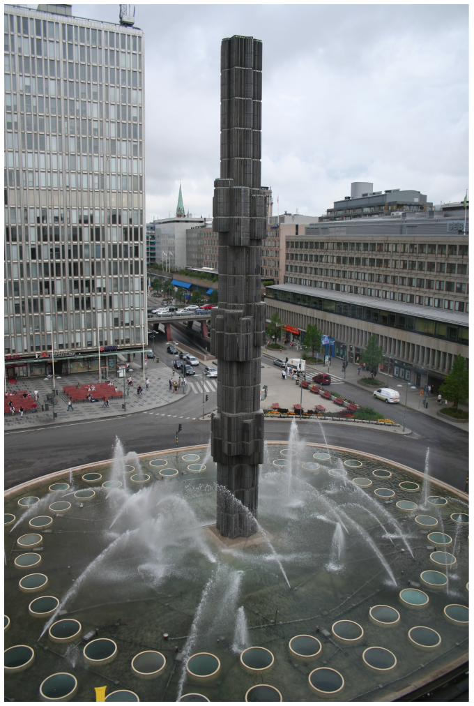
To draw the Lamé curve it is preferable we use the following parametric formulation.
\[\left\{ \begin{aligned} x\left(t\right) &= a\left(\cos^2 t\right)^{\frac{1}{n}} \cdot \sgn \cos t\\ y\left(t\right) &= b\left(\sin^2 t\right)^{\frac{1}{n}} \cdot \sgn \sin t \end{aligned}\right. \qquad -\pi \le t < \pi\]
The translation of this formula to Julia is direct:
super_ellipse(p, a, b, n, t) =
p+vxy(a*(cos(t)^2)^(1.0/n)*copysign(1, cos(t)), b*(sin(t)^2)^(1.0/n)*copysign(1, sin(t)))
In order to generate a sequence of points of the superellipse we can, as previously, use the map_division function:
superellipse_points(p, a, b, n, pts) =
map(t -> super_ellipse(p, a, b, n, t),
division(-pi, pi, pts))
Finally, to plot the superellipse, we can define:
superellipse_curve(p, a, b, n, pts) =
spline(superellipse_points(p, a, b, n, pts))
The superellipses in this figure were generated using the previous function. For this, we defined a function test_superellipses which, for values of \(a\) and \(b\) and for a sequence of numbers, tests all the combinations of exponent \(n=p/q\), with \(p\) and \(q\) taking successive values from that sequence. For viewing the super-ellipses each of them has an origin proportional to the combination used of \(p\) and \(q\):
test_superellipses(a, b, ns) =
for num in ns
for den in ns
superellipse_curve(xy(num*2.5*a, den*2.5*b), a, b, num/den, 100)
end
end
This figure was directly generated from the evaluation of the following expression:
test_superellipses(2.0, 1.0, [1, 2, 3, 4, 5, 6, 7, 8])
10.4.7 Exercises 47
10.4.7.1 Question 182
Define the function tank_superellipse that creates a tank with a superelliptical shape identical to the one of Sergels Torg’s square, as presented below:
Suggestion: define a function named curved_wall that builds walls along a given curve. The function should receive the thickness and height of the wall and an entity representing the curve (e.g., a circle, a spline, etc.). Consider using the function sweep defined in section Extrusions as well.
10.4.7.2 Question 183
Define the function circular_tanks that builds a succession of circular tanks of which the centers are located along a superellipse, as presented in the following image:
The function should receive the parameters of the superellipse, the parameters of a circular tank and the number of tanks to create.
10.4.7.3 Question 184
Define a function that, by invoking the functions tank_superellipse and circular_tanks, creates a square as similar as possible to Sergels Torg’s square, as shown in the following figure:
10.4.7.4 Question 185
Modify the previous function to produce a variant that is perfectly circular:
10.4.7.5 Question 186
Modify the previous function to produce the following variant:
10.4.7.6 Question 187
Modify the previous functions to produce the following variant:
10.5 Precision
Let us consider the butterfly curve, proposed by the mathematician Temple H. Fay. This periodic curve is defined by the following equation in polar coordinates:
\[r=e^{\sin \phi} - 2 \cos (4 \phi ) + \sin^5\left(\frac{2 \phi - \pi}{24}\right)\]
Similar to what we did before, we will consider the curve with respect to a starting point \(P\), within a range of variation of the independent parameter \(t \in [t_0, t_1]\).
butterfly_curve(p, t0, t1, n) =
map(t -> p+vpol(exp(sin(t))+-2*cos(4*t)+sin((2*t-pi)/24)^5, t),
division(t0, t1, n, false))
To draw this curve we are left with determining the appropriate value of the parameter \(n\). For this, it is important to realize that the period of the Butterfly curve is \(24 \pi\), with the entire curve generated for \(t \in [0, 24\pi]\). Since this period is relatively large, the number \(n\) of points to be used should be enough so that the curve can be accurately reproduced and it is precisely here that the greatest difficulty arises: without knowing the shape of the curve, it is difficult to estimate which is the best value for \(n\). If the value of \(n\) is too low, the curve will not be faithfully represented, in particular, in places where there are very accentuated curvatures; if the value is too high, the greater the need for computational resources. In practice, some experimentation is required to understand what best value is.
This need for experimentation relative to the value of number of points to be used is clearly evident in this figure which shows the Butterfly curves drawn for the following increasing values of \(n\):
closed_spline(butterfly_curve(xy(0, 10), 0, 24*pi, 10))
closed_spline(butterfly_curve(xy(10, 10), 0, 24*pi, 20))
closed_spline(butterfly_curve(xy(20, 10), 0, 24*pi, 40))
closed_spline(butterfly_curve(xy(30, 10), 0, 24*pi, 80))
closed_spline(butterfly_curve(xy(40, 10), 0, 24*pi, 160))
closed_spline(butterfly_curve(xy(0, 0), 0, 24*pi, 320))
closed_spline(butterfly_curve(xy(10, 0), 0, 24*pi, 640))
closed_spline(butterfly_curve(xy(20, 0), 0, 24*pi, 1280))
closed_spline(butterfly_curve(xy(30, 0), 0, 24*pi, 2560))
closed_spline(butterfly_curve(xy(40, 0), 0, 24*pi, 5120))
The butterfly curve produced for increasing values of the number \(n\) of points.
As we can verify, when the number of points is insufficient, the produced curves can be grotesque distortions of reality. For this reason, we should take particular care in choosing the value most suitable for this parameter.
An interesting alternative is to give the computer the responsibility of adapting the number of points to the necessities of each curve.
10.5.1 Adaptive Sampling
The map_division function allows us to generate the curve of any function \(f(t)\) in the interval \([t_0, t_1]\) by applying the function \(f\) to a sequence of \(n\) increments of \(t\) equally spaced \(\{t_0,\ldots,t_1\}\). This sequence is named sampling sequence.
It is easy to see that the greater the number of the sampling sequence elements, the greater the accuracy of the produced curve will be. Unfortunately, the greater that accuracy, the greater the effort expended for computing the function values in all elements of the sequence. In practice, it is necessary we find a balance between accuracy and computational effort.
Unfortunately, there are several functions for which it is difficult or even impossible to find an appropriate number of sampling points. As an example, let us try to produce the graph of the function \(f(t)=(t,\frac{1}{2}sin(\frac{1}{t}))\) in the interval \([0.05,0.8]\). This function has a curve for a graph that oscillates with a frequency that is greater the closer it is to the origin. This figure shows a sequence of graphs of this function in which, from left to right, the number of sampling points was progressively increased.
Graph of the function \(f(x)=\frac{1}{2}sin(\frac{1}{x})\) in the interval \([0.05,0.8]\). From left to right the sampling points \(8,15,30\) and \(60\) were employed.
As we can see in the figure, with few sampling points the resulting curve is a grotesque approximation of the real curve and it is only when the number of sampling points becomes very high that some precision is acquired. It so happens that that precision is only relevant in parts of the curve where there are large variations. In other areas where the curve evolves "smoothly" more sampling points only imply greater processing time, without any significant advantage to the quality of the result. This suggests that we should adapt the number of sampling points along the curve according to its "smoothness": in areas where the curve varies more sharply we should employ more sampling points, but in areas where the variation is more linear, we can decrease the number of sampling points. This way, the number of sampling points adapts to shape of the curve.
Adaptive generation of points
For us to employ an adaptive sampling we need to define a criteria to classify the "smoothness" of a curve. As illustrated in this figure, we can start by admitting that we have two abscissae \(x_0\) and \(x_1\) that we use to calculate the points \(P_0\) and \(P_1\). To know if the curve behaves in a linear fashion between those two points (and thus can be approximated by a line segment), we shall calculate the average value \(x_m\) of that interval and the corresponding point \(P_m\) of the curve. If the function is in fact linear in that interval, then the points \(P_a\) and \(P_m\) are collinear. In practice, that will rarely happen, so we will have to use a concept of approximate collinearity, for which we can use any of the several possible criteria, such as:
The area of the triangle \(P_0,P_m,P_1\) to be smaller than a sufficiently small value of \(\epsilon\) .
The angle \(P_0,P_m,P_1\) to be approximately equal to \(\pi\).
The sum of the distance between \(P_0\) and \(P_m\) with the distance between \(P_m\) and \(P_1\) to be approximately equal to the distance between \(P_0\) and \(P_m\).
Other criteria would be equally applicable, but for now, let us choose the first. Its translation into Julia is as follows:
isapproximately_collinear(p0, pm, p1, epsilon) =
let (a, b, c) = (distance(p0, pm), distance(pm, p1), distance(p1, p0))
area_triangle(a, b, c) < epsilon
end
area_triangle(a, b, c) =
let s = (a+b+c)/2.0
sqrt(s*(s-a)*(s-b)*(s-c))
end
The isapproximately_collinear function implements the criteria that allows us to say that the line segments connecting the points p0, pm, and p1 are a good approximation to the curve’s behavior between those points. When this criteria does not occur, we can split the interval into two sub-intervals, and analyze each of them separately, concatenating the results.
map_division_adapt(f, t0, t1, epsilon) =
begin
p0 = f(t0)
p1 = f(t1)
tm = (t0+t1)/2.0
pm = f(tm)
isapproximately_collinear(p0,
pm,
p1,
epsilon) ?
[p0, pm, p1] :
[map_division_adapt(f, t0, tm, epsilon)...,
map_division_adapt(f, tm, t1, epsilon)[2:end]...]
end
This adaptive way of producing a sample of a curve allows results with greater precision even when employing a relatively small total number of sampling points. This figure shows a sequence of graphs identical to those shown in this figure, but now using an adaptive sampling scheme with approximately the same number of sampling points in each case. As we can see, the graphs are substantially more accurate, particularly in areas close to the origin, without this visibly diminishing the quality of the curve in areas where the change is smoother.
Graph of the function \(f(x)=\frac{1}{2}sin(\frac{1}{x})\) in the interval \([0.05,0.8]\). From left to right, the sequence of adaptive sampling has, respectively, \(7,15,29\) and \(57\) points.
10.5.2 Exercises 48
10.5.2.1 Question 188
The algorithm used in the map_division_adapt function can not properly deal with periodic functions in which we have \(f(t_0)=f(t_1)=f(\frac{t_0+t_1}{2})\). In this case, the degenerate triangle formed by these three points has zero area, which makes the algorithm terminate immediately. Modify the function so it receives an additional parameter \(\Delta_T\) that determines the biggest admissible interval between two consecutive values of \(t\).
10.5.2.2 Question 189
The map_division_adapt function is not as efficient as it could be, in particular, because it systematically repeats the application of the function \(f\) at the midpoint: \(f(t_m)\) is calculated to decide whether the recursion continues and, when it continues, it will have to be calculated again to allow calculating \(f(t_0)\) or \(f(t_1)\) on the following call. Redefine the map_division_adapt function in order to avoid repetitive calculations.
10.6 Parametric Surfaces
Throughout history, architecture has explored a huge variety of forms. As we have seen, some of these forms correspond to solids well known since antiquity, such as cubes, spheres and cones. More recently, architects have turned their attention for much less classical forms, which require a different kind of description. The famous Spanish architect Felix Candela is a good example.
Candela thoroughly explored the properties of the hyperbolic paraboloid, allowing him to create works that are now references in the world of architecture. This figure illustrates the construction of one of the works by Félix Candela, where the fundamental element is precisely a thin concrete shell in the shape of a hyperbolic paraboloid. In his time, Candela performed all necessary calculations manually to determine the forms he intended to create. We will now see how we can get the same results in a much more efficient way.
The Lomas de Cuernavaca Chapel under construction. Photograph by Dorothy Candela.
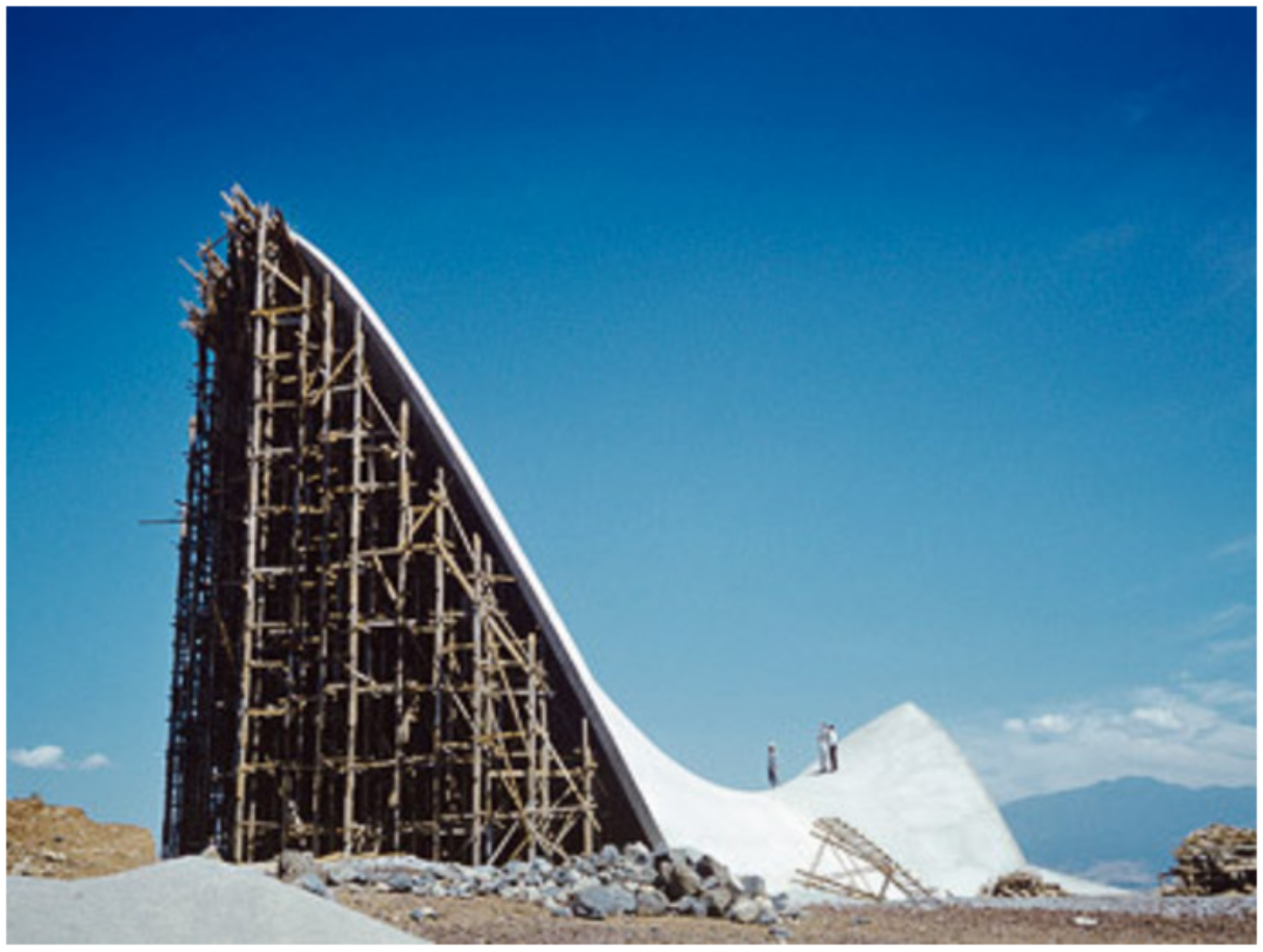
Mathematically speaking, a parametric surface is simply the image of an injective function of \(\mathbb R^2\) in \(\mathbb R^3\).
As it happens with curves, although we can describe a surface in an implicit form, the parametric representation is more adequate for the generation of the positions through which the surface passes. For example, a sphere centered at point \((x_0, y_0, z_0)\) and with radius \(r\), can be described implicitly by the equation
\[(x-x_0)^2+(y-y_0)^2+(z-z_0)^2-r^2=0\]
but this form does not allow the direct generation of coordinates, being more preferable the adoption of a parametric description, by the functions
\[\left\{ \begin{aligned} x(\phi,\psi) &= x_0 + r \sin\phi\cos\psi\\ y(\phi,\psi) &= y_0 + r \sin\phi\sin\psi\\ z(\phi,\psi) & =z_0 + r \cos\phi \end{aligned}\right.\]
The Möbius Strip is not a true surface, but a surface with boundary.
10.6.1 The Möbius Strip
This property has been exploited, for example, in transmission belts that, when adopting the topology of a Möbius strip, they wear out both "sides" of the belt instead of only one, thereby making them last twice as long.
The Möbius Strip.
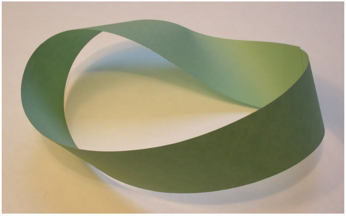
The Möbius strip has been successively used in various contexts, from the famous works of Maurits Cornelis Escher that employ a Möbius strip, as "Möbius Strip II", to the representative symbol of the recycling, which consists of three arrows arranged along a Möbius strip, as can be see in this figure.
The representative symbol of recycling: three arrows arranged along a Möbius strip.

The parametric equations of this surface, in cylindrical coordinates, are as follows:
\[\left\{ \begin{aligned} \rho(s,t)& =1 + t \cos\frac{s}{2}\\ \theta(s,t)& =s\\ z(s,t)& =t \sin\frac{s}{2} \end{aligned}\right.\]
Given the periodicity of the trigonometric functions, we have that \(\frac{s}{2} \in [0,2\pi]\) or \(s \in [0,4\pi]\). In that period, for a given \(t\), the \(z\) coordinate will assume symmetrical values in relation to the \(xy\) plane, in the limit, between \(-t\) and \(t\). This means that the Möbius strip develops up and down the \(xy\) plane.
To draw this surface we can use, as an initial approach, a generalization of the process we used to draw parametric curves. In this approach, we simply applied the argument function \(f(t)\) along a succession of \(n\) values from \(t_0\) to \(t_1\). In the case of parametric surfaces, we intend on applying the function \(f(s,t)\) over a succession of \(m\) values from \(s_0\) to \(s_1\), and for each one, over a succession of \(n\) values, from \(t_0\) to \(t_1\). Thus, the \(f(s,t)\) function will be applied to \(m\times n\) pairs of values. This behavior is easily obtained at the expense of two chained mappings:
map(s -> map(t -> f(s, t), division(t0, t1, n)),
division(s0, s1, m))
For example, in the case of Möbius strip, we can define:
mobius_strip(s0, s1, m, t0, t1, n) =
map(s -> map(t -> cyl(1+t*cos(s/2), s, t*sin(s/2)), division(t0, t1, m)),
division(s0, s1, n))
In fact, this combination of mappings with interval divisions is so frequent that Rosetta already provides it through an extension of the map_division function, allowing us to write
mobius_strip(s0, s1, m, t0, t1, n) =
map_division((s, t) -> cyl(1+t*cos(s/2), s, t*sin(s/2)), s0, s1, m, t0, t1, n)
We have seen that in the case of a function with a single parameter \(f(t)\), we had that
map_division(unsyntax(lispemph(f)),
unsyntax(lispemphi(t, "0")),
unsyntax(lispemphi(t, "1")),
unsyntax(lispemph(n)))
map(unsyntax(lispemph(f)),
division(unsyntax(lispemphi(t, "0")),
unsyntax(lispemphi(t, "1")),
unsyntax(lispemph(n))))
This equivalence is now extended to the case of functions that have two parameters \(f(s,t)\), that is,
map_division(unsyntax(lispemph(f)),
unsyntax(lispemphi(s, "0")),
unsyntax(lispemphi(s, "1")),
unsyntax(lispemph(m)),
unsyntax(lispemphi(t, "0")),
unsyntax(lispemphi(t, "1")),
unsyntax(lispemph(n)))
is equivalent to
map(s -> map(t -> unsyntax(lispemph(f))(s, t), division(unsyntax(lispemphi(t, "0")), unsyntax(lispemphi(t, "1")), unsyntax(lispemph(n)))),
division(unsyntax(lispemphi(s, "0")),
unsyntax(lispemphi(s, "1")),
unsyntax(lispemph(m))))
Naturally, if the interior mapping produces a list with the results of the application of the function \(f\), the exterior mapping will produce a list of lists of results of the application of the function \(f\). Assuming that each application of the function \(f\) yields a point in three-dimensional coordinates, we can easily see that this expression produces a list of lists of points. Thus, the result will be in the form of:
unsyntax(lispemphi(P, "0,0"))(unsyntax(lispemphi(P, "0,1")), ___, unsyntax(lispemphi(P, "0,m")))(unsyntax(lispemphi(P, "1,0"))(unsyntax(lispemphi(P, "1,1")),
___,
unsyntax(lispemphi(P, "1,m"))),
___,
unsyntax(lispemphi(P, "n,0"))(unsyntax(lispemphi(P, "n,1")),
___,
unsyntax(lispemphi(P, "n,m"))))
To draw this list of lists of points, we can simply apply the spline function to each of the lists of points:
splines(ptss) = map(spline,
ptss)
Thus, we can easily represent a first preview of the Möbius strip:
splines(mobius_strip(0, 4*pi, 80, 0, 0.3, 10))
The result of the evaluation of the above expression is represented in this figure.
The Möbius strip.
An interesting aspect of three-dimensional parametric surfaces is that the set of points that define them can be arranged in a matrix. In fact, if the parametric surface is obtained by applying the function \(f(s,t)\) over a succession of \(m\) values, from \(s_0\) to \(s_1\), and for each one, over a succession of \(n\) values from \(t_0\) to \(t_1\), we can place the results of those applications in a matrix of \(m\) rows and \(n\) columns, as follows:
\[\begin{bmatrix} f(s_0,t_0) & \dots & f(s_0,t_1)\\ \dots & \dots & \dots\\ f(s_1,t_0) & \dots & f(s_1,t_1) \end{bmatrix}\]
What the map_division function returns is nothing more than a representation of this matrix, implemented in terms of a list of matrix rows, each row implemented in terms of a list of values corresponding to the elements of that row of the matrix.
It is now easy to see that the application of the function splines to the representation of the matrix does nothing else than to draw \(m\) splines, each defined by \(n\) points of each of the \(m\) rows of the matrix. Another alternative is to draw \(n\) splines defined by \(m\) points of each of the \(n\) columns of the matrix. For this, the simplest way is to transpose the matrix, i.e., change the lines with the columns, in the form:
\[\begin{bmatrix} f(s_0,t_0) & \dots & f(s_1,t_0)\\ \dots & \dots & \dots\\ f(s_0,t_1) & \dots & f(s_1,t_1) \end{bmatrix}\]
For this, we can define a function that, given a matrix implemented as a list of lists, returns the transposed matrix in the same implementation:
transposed_matrix(matrix) =
matrix[1] == [] ?
[] :
[map(l -> l[1], matrix), transposed_matrix(map(l -> l[2:end], matrix))...]
Using this function, it is now possible to trace orthogonal curves to the ones represented in this figure simply by tracing the obtained curves from the transposed matrix, i.e.
splines(transposed_matrix(mobius_strip(0, 4*pi, 80, 0, 0.3, 10)))
The Möbius strip.
The result is shown in this figure.
Finally, to obtain a mesh with the combined effect of both curves, we can define an auxiliary function mesh_splines:
mesh_splines(ptss) =
begin
splines(ptss)
splines(transposed_matrix(ptss))
end
We can now use this function as follows:
mesh_splines(mobius_strip(0, 4*pi, 80, 0, 0.3, 10))
The Möbius strip.
The result is shown in this figure.
This type of representation based on the use of lines to give the illusion of an object, is called wireframe. Formally, a wireframe is nothing more than a set of lines that represent a surface. Wireframe models have the advantage, over other forms of visualization, of allowing a much faster drawing.
10.7 Surfaces
Wireframe models do not constitute surfaces. In fact, as the lines are infinitely thin and there is no "material" between them, it is not possible to associate a wireframe model to a real surface.
If what we want is, in fact, to draw surfaces, then it is preferable we exploit the capabilities of Rosetta for the creation of surfaces.
Polygon meshes are clusters of polygons, usually triangles and quadrilaterals which define the shape of an object. In comparison to models constituted only by lines, polygon meshes have the advantage of being more realistically displayed, for example, with the removing of invisible surfaces, with the inclusion of shading, etc. Obviously, each face of these polygonal meshes has zero thickness, therefore they are not actually solids but only abstract representations of surfaces. Even so, they can be very useful to obtain a more correct visualization of a surface and can be subsequently transformed for creating solids, for example, using the function thicken that gives the surface a uniform thickness.
Rosetta provides an operation for creating these polygonal meshes named surface_grid. This figure shows a realistic representation of the Möbius strip generated from the following expression:
surface_grid(mobius_strip(0, 4*pi, 80, 0, 0.3, 10))
The Möbius strip.
It is now trivial to experiment with variations of the Möbius strip, for example, to vary the strip’s "width", as depicted in this figure.
The Möbius strip for different "widths". From left to right the variation interval in \(v\) is \([0,\frac{1}{2}]\), \([0,1]\), \([0,2]\) and \([0,4]\).
To visualize a more architectural example, let us consider the hyperbolic paraboloid used by Félix Candela in the Lomas Cuernavaca Chapel. This surface can be described in its implicit representation by the equation
\[x^2-y^2-z=0\]
or, likewise, through its parametric representation:
\[\left\{ \begin{aligned} x(s,t)& = s\\ y(s,t)& = t\\ z(s,t)& = s^2 - t^2 \end{aligned}\right.\]
The translation to Rosetta is trivial:
thicken(surface_grid(map_division((x, y) -> xyz(x, y, x*x-y*y),
-0.5,
1.3,
40,
-2,
2,
80)),
0.03)
In the previous expression, we used the domain limits that approximate the surface to the real work and we gave thickness to the surface through the function thicken. In this figure we show a view of the work where we eliminated the portion that is under the earth.
An approximation of the Lomas Cuernavaca Chapel.
10.7.1 Exercises 49
10.7.1.1 Question 190
Define a function that, with appropriate arguments, builds the surface shown in the following figure.
10.7.1.2 Question 191
Consider the following image:
Assume that the figure is centered at the origin and represented using an isometric perspective. Notice that the surface intersections with any plane parallel to the \(XZ\) plane or to the \(YZ\) plane produces a perfect sinusoid (though it produces sinusoids of different frequencies depending on the distance from the intersection plane to the origin). From these tips, try to figure out the parametric equations that originated it.
10.7.2 Helicoid
We discussed, in section (part "sec:helix"), the drawing of the helix. Let us now discuss the surface that generalizes this curve: the helicoid.
The helicoid was discovered in 1776 by Jean Baptiste Meusnier. Its parametric equations (in cylindrical coordinates) are:
\[\left\{ \begin{aligned} \rho(u,v)& =u\\ \theta(u,v)& =\alpha v\\ z(u,v)& =v \end{aligned}\right.\]
This figure shows two helicoids with different parameters, generated from the following fragment of program:
Two helicoids with variation intervals in \(v\) of \([0,2\pi]\). The left helicoid has \(\alpha=1\), and variation interval in \(u\) of \([0,1]\) while the right one has \(\alpha=3\) and \(u \in [0,5]\).
helicoid(p, a, u0, u1, m, v0, v1, n) =
map_division((u, v) -> p+vcyl(u, a*v, v), u0, u1, m, v0, v1, n)
surface_grid(helicoid(xyz(0, 0, 0), 1, 0, 1, 10, 0, 2*pi, 100))
surface_grid(helicoid(xyz(7, 0, 0), 3, 0, 5, 50, 0, 2*pi, 200))
An interesting feature of the helicoid is that for each point of the helicoid there is a helix that passes though it.
10.7.3 Spring
A spring is another geometric figure that has affinities with an helix. Mathematically, the spring is the volume generated by a circle that travels along an helix. In simpler terms, a spring is an helix with "thickness", i.e., a tube that wraps around an axis. If \(r_0\) is the radius of the tube, \(r_1\) the distance from the tube axis to the helix axis, \(\alpha\) the initial rotation angle of the spring and \(v_z\) the "speed" along the \(z\) axis, the parametric equations of the spring are:
\[\left\{ \begin{aligned} \rho(u,v)& =r_1+r_0\cos u\\ \theta(u,v)& =\alpha+v\\ z(u,v)& = \frac{v_z v}{\pi} + r_0\sin u \end{aligned}\right.\]
The translation of the above definition into Julia is:
spring(p, a, r0, r1, vz, u0, u1, m, v0, v1, n) =
map_division((u, v) -> p+vcyl(r1+r0*cos(u), a+v, (vz*v)/pi+r0*sin(u)),
u0,
u1,
m,
v0,
v1,
n)
In this figure we find visualizations of a spring in its extension process. Each image corresponds to a spring with the same dimensions, except in regards to the "speed" in \(z\).
surface_grid(spring(xyz(0, 0, 0), 0, 1, 5, 1, 0, 2*pi, 50, 0, 3*2*pi, 150))
surface_grid(spring(xyz(20, 0, 0), 0, 1, 5, 2, 0, 2*pi, 50, 0, 3*2*pi, 150))
surface_grid(spring(xyz(40, 0, 0), 0, 1, 5, 4, 0, 2*pi, 50, 0, 3*2*pi, 150))
Three springs created with the parameters \(r_0=1\), \(r_1=5\), \(u \in [0, 2\pi]\) and \(v \in [0, 6\pi]\). From left to right, we have the speed \(vz \in \{1,2,4\}\).
10.7.4 Exercises 50
10.7.4.1 Question 192
The traditional spring is just the simplest form that is possible to generate from the function spring. More elaborate shapes can be generated by either parametrization, or by composition. For example, by composing "springs" we can generate ropes. In this case, we treat the "springs" as "strands" or "filaments" which, wrapped around each other, constitute a rope.
Thus, a rope can be seen as a set of intertwined springs, with all the springs developing along the same axis but "rotated" (i.e., with an initial angle) and a step (i.e., a velocity of development) which allows them to be close to each other. In the following Figure we have represented two schemes that show, on the left, the position of the springs in the case of a rope with four "strands". This rope can be generalized from any number of strands, to the lower limit of two strands, shown on the right.
Define the function rope that, by receiving the appropriate parameters, creates ropes. For example, consider the following expressions of which the evaluation produces three ropes built with two, three and six strands, shown below:
rope(xyz(0, 0, 0), 2, 1, 3)
rope(xyz(10, 0, 0), 3, 1, 2)
rope(xyz(20, 0, 0), 6, 1, 1)
10.7.4.2 Question 193
A breather is a mathematical surface that characterizes a particular type of wave which is illustrated in the following Figure. Its parametric equation is::
\[\left\{ \begin{aligned} x(u,v)& = -u+\frac{2\left(1-a^2\right)\cosh(au)\sinh(au)}{a\left(\left(1-a^2\right)\cosh^2(au)+a^2\,\sin^2\left(\sqrt{1-a^2}v\right)\right)} \\ y(u,v)& = \frac{2\sqrt{1-a^2}\cosh(au)\left(-\sqrt{1-a^2}\cos(v)\cos\left(\sqrt{1-a^2}v\right)-\sin(v)\sin\left(\sqrt{1-a^2}v\right)\right)}{a\left(\left(1-a^2\right)\cosh^2(au)+a^2\,\sin^2\left(\sqrt{1-a^2}v\right)\right)} \\ z(u,v)& = \frac{2\sqrt{1-a^2}\cosh(au)\left(-\sqrt{1-a^2}\sin(v)\cos\left(\sqrt{1-a^2}v\right)+\cos(v)\sin\left(\sqrt{1-a^2}v\right)\right)}{a\left(\left(1-a^2\right)\cosh^2(au)+a^2\,\sin^2\left(\sqrt{1-a^2}v\right)\right)} \end{aligned}\right.\]
Note that due to the periodicity of the trigonometric functions, we have that \(-2\pi\leq u \leq 2\pi\) and \(-12\pi\leq v \leq 12\pi\). The \(a\) parameter characterizes different surfaces and may vary between \(0\) and \(1\).
Define the function breather that draws the surface in question from a point \(P\), the parameter \(b\) and the variation limits and the number of points to consider along that variation, respectively, for the parameters \(u\) and \(v\). For example, the previous figure was produced by evaluating the expression:
surface_grid(breather(xyz(0, 0, 0), 0.4, -13.2, 13.2, 200, -37.4, 37.4, 200))
10.7.5 Shells
Several authors argue that nature is a mathematical manifestation and justify this belief by the striking resemblance that some mathematical surfaces exhibit with natural forms.
The Dini surface, is one such cases. The parametric equations that define it are:
\[\left\{ \begin{aligned} x(u,v)& =\cos(u)\sin(v)\\ y(u,v)& =\sin(u)\sin(v)\\ z(u,v)& =\cos(v)+\log(\tan(\frac{v}{2}))+a*u \end{aligned}\right.\]
where \(0\leq u\leq 2\pi\) and \(0\leq v\leq\pi\).
The translation of these equations into Julia is direct:
dini(p, a, u0, u1, m, v0, v1, n) =
map_division((u, v) -> p+vxyz(cos(u)*sin(v), sin(u)*sin(v), cos(v)+log(tan(v/2.0))+a*u),
u0,
u1,
m,
v0,
v1,
n)
The following invocations of this function show how it is possible, in fact, to simulate the natural shapes of certain types of shells. The result is represented in this figure.
surface_grid(dini(xyz(0, 0, 0), 0.2, 0, 6*pi, 100, 0.1, pi*0.5, 100))
surface_grid(dini(xyz(3, 0, 0), 0.2, 0, 6*pi, 100, 0.1, pi*0.7, 100))
surface_grid(dini(xyz(6, 0, 0), 0.2, 0, 6*pi, 100, 0.1, pi*0.9, 100))
The Dini surface as a mathematical approximation of the form of certain types of shells.
Another example is the spiral shell, defined mathematically (in Julia) by:
shell(p, a, b, u0, u1, m, v0, v1, n) =
map_division((u, v) -> let (e, c) = (exp(u/6.0/pi), cos(v/2.0)^2); p+vxyz(a*(1-e)*cos(u)*c, b*(e-1)*sin(u)*c, 1-exp(u/3.0/pi)-sin(v)+e*sin(v)) end,
u0,
u1,
m,
v0,
v1,
n)
From the previous function, we can experiment variations like the ones presented below, and which generate the surfaces represented in this figure.
surface_grid(shell(xyz(0, 0, 0), 1, 1, 0, 7*pi, 100, 0, 2*pi, 100))
surface_grid(shell(xyz(7, 0, 0), 2, 2, 0, 7*pi, 100, 0, 2*pi, 100))
surface_grid(shell(xyz(18, 0, 0), 3, 1, 0, 7*pi, 100, 0, 2*pi, 100))
A mathematical approximation of the shape of spiral shells.
10.7.6 Cylinders, Cones, and Spheres
Although we have illustrated the previous section with relatively complex surfaces, in this section we will start by doing surface that are comparatively much simpler, which will allow us to realize that the parametric construction of surfaces is relatively easy as long as we understand the impact of the variation of the independent parameters \(u\) and \(v\).
For example, the surface of a cylinder of radius \(r\) is characterized by being the set of points that are at a fixed distance \(r\) of an axis and from a minimum \(h_0\) and maximum \(h_1\) "height" relative to that axis.
Assuming, for simplicity, that we will match the cylinder axis with the \(Z\) axis, this means that we employ cylindrical coordinates \((\rho, \phi,z)\), with the cylinder surface being defined simply by fixing \(\rho=r\) and letting \(\phi\) vary between \(0\) and \(2\pi\) and \(z\) vary between \(h_0\) and \(h_1\). With \(\rho\) being fixed and the variations of \(\phi\) and \(z\) being independent, the use of parametric surfaces is trivial: we need only use one of the parameters \(u\) or \(v\) to make the variation of \(\phi\) and the other for the variation of \(z\).
More specifically, let us make \(\rho(u,v)=r\) and let \(\phi(u,v)=u\) and \(z(u,v)=v\) vary independently, respectively between \(u\in [0,2\pi]\) and \(v\in [h_0,h_1]\). Since \(\phi\) depends directly and exclusively on \(u\) and \(z\) depends directly and exclusively on \(v\), we can use these parameters directly in the function. This way, we are able to write a function that produces a cylindrical coordinate from the value of the radius \(r\) and from the independent parameters \(\phi\) and \(z\).
The image on the left in this figure shows the cylinder of radius \(1\) between \(h_0=-1\) and \(h_1=1\), produced by the evaluation of following expression:
surface_grid(map_division((phi, z) -> cyl(1, phi, z), 0, 2*pi, 60, -1, 1, 20))
If, instead of fixing the radius of \(\rho(phi,z)=r\), we make it vary in function to the height \(z\), then it is obvious that the radius of the "cylinder" will be zero at the origin and will increase (in absolute value) as it moves away from the origin. The only difference to the previous case will thus be on the expression that creates the cylindrical coordinates, which will now be cyl(z, phi, z), reflecting the linear increase of the radius with \(z\). Evidently, the resulting figure will not be a cylinder but a cone, that we present in the central image of this figure.
Finally, let us consider the description of a sphere of radius \(r\) in spherical coordinates \((\rho, \phi, \psi)\), which is reduced to \(\rho=r\), with \(\phi\) varying between \(0\) and \(2\pi\) and \(\psi\) varying between \(0\) and \(\pi\). Once again, we need two independent variations, for which we can arbitrarily assign \(u\) to one and \(v\) to the another. Thus, let us make \(\rho(u,v)=r\), \(\phi(u,v)=u\) and \(\psi(u,v)=v\) with \(u\in [0,2\pi]\) and \(v\in [0,\pi]\). As is was did in the two previous examples, this association between \(\phi\) and \(\psi\) and, respectively, \(u\) and \(v\), allows us to write the function directly in terms of the former. Exemplifying with \(r=1\), we have:
surface_grid(map_division((phi, psi) -> sph(1, phi, psi),
0,
2*pi,
60,
0,
pi,
30))
The result is on the right of this figure.
A cylinder, a cone and a sphere generated as parametric surfaces.
To see the impact that small changes in parameters can have on the shape of generated surfaces, let us try three variations on the shape of the sphere. The first variation is to add to the radius of the sphere a sinusoid with high frequency and low amplitude, in terms of "latitude" \(\psi\), for example, by making \(\rho=1+\frac{\sin(20\psi)}{20}\). The result will be a formation of waves from pole to pole, as is visible in the image on the right of this figure. If, on the other hand, we decide to make the same change in radius to be dependent on an identical sinusoid but in terms of \(\phi\), then the waves travel along the "longitude", for example, from east to west. This effect is illustrated on the central image of this figure. Finally, we can get a combined effect by making the radius simultaneously dependent on a sinusoid in terms of "latitude" and other sinusoid in terms of "longitude", i.e., \(\rho=1+\frac{\sin(20\phi)}{20}+\frac{\sin(20\psi)}{20}\). The result is shown on the right image of this figure.
Spheres of which the radius is a function of the "latitude", "longitude" or both.
10.7.7 Exercises 51
10.7.7.1 Question 194
Consider the following ellipsoid:
An ellipsoid is characterized by the dimensions of its three orthogonal radii \(a\), \(b\) and \(c\). Its parametric equation is:
\[\begin{aligned} x&=a\sin \psi \cos \phi\\ y&=b\sin \psi \sin \phi\\ z&=c\cos \psi\end{aligned}\] \[\begin{matrix}-\frac{\pi}{2}\leq\phi\leq+\frac{\pi}{2};\quad-\pi\leq\psi\leq+\pi;\end{matrix}\]
Define the ellipsoid function that produces the ellipsoid from the three radii \(a\), \(b\), \(c\), and also from the number \(n\) of values to use along \(\phi\) and \(\psi\).
10.8 Bodegas Ysios
The Bodegas Ysios is a building designed by Santiago Calatrava and intended for the production, storage and distribution of wines. this figure shows a front view of the building.
Bodegas Ysios. Photograph by Luis Antonio Ortuño.
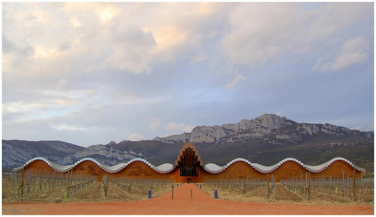
The opposing phases means that when one of the sinusoids reaches its maximum value, the other reaches its minimum and vice versa. For this to happen, the difference between phases of the two sinusoids has to be \(\pi\).
As can be seen in this figure, the central part of the south facade, intended to accommodate the visitor center, is more prominent and higher than the rest of the building.
As shown in this figure, the roof parallelepipeds are made of aluminium, in contrast with the cedar wood that is used on the south facade. On the north facade, concrete is used with some small openings for illumination. The east and west facades consist of wavy aluminium plates.
Bodegas Ysios. Photograph by Koikile.
In this section we will address the modeling of the frontal wall of the wine cellar. In a first analysis, we can model this wall as a vertical extrusion of a sinusoid. Unfortunately, although this operation can properly model the lateral sides of the wall, it can not do so for the central part because, in this area, the wall has a more complex evolution that moves away from the vertical.
A second approach could be the interpolation of regions, but this will only be achievable if we can shape the curves that delimit the wall. In addition to that, a large number of curves may be necessary in order to accurately represent the surface of the wall.
A third approach, more rigorous, consists in the mathematical description of the surface in question. This way, the required "curves" could be generated automatically. While it may be difficult to see at first glance that the wall of Bodegas Ysios can be modeled by a mathematical function, we will see that it is relatively simple to undertake this modeling through the composition and modification of simpler functions.
As a first approximation, we can start by considering a sinusoidal wall identical to what we would get if we were to make a vertical extrusion of a sinusoid. For simplicity, we will center the wall base at the origin, which implies that the central hump has its maximum amplitude at the origin. Seeing as the sine amplitude is zero at the origin, this suggests that instead of a sine, it is preferable we use a cosine, of which the amplitude is maximum at the origin. The observation of this work by Calatrava indicates that this cosine performs three cycles for each side, for which the period should range between \(-6\pi\) and \(+6\pi\). Admitting that this wall evolves along the \(XZ\) plane, we can start by experimenting the following expression:
surface_grid(map_division((x, z) -> xyz(x, cos(x), z),
-7*pi,
7*pi,
100,
0,
5,
10))
The expression shows that we make the \(x\) coordinate vary freely with \(u\), we make the \(y\) coordinate be the \(x\) cosine, and finally we make the \(z\) coordinate vary freely with \(v\). As we can observe in this figure, the surface is a good approximation of the lateral sides of the front wall of the Bodegas Ysios.
First approach to modeling the Bodegas Ysios.
Let us now model the sinusoids at the top of the wall, where the roof’s parallelepipeds are supported. For this, we will simply "deform" the surface, causing the \(z\) coordinate to oscillate in a cos-sinusoidal way along the \(x\) axis, increasing the oscillation amplitude as we go up in \(z\). In order for the wall to have its base free of the influence of this cos-sinusoid, we will raise the cosine by one unit and use a reduced initial amplitude:
surface_grid(map_division((x, z) -> xyz(x, cos(x), z*(1+0.2*cos(x))),
-7*pi,
7*pi,
100,
0,
5,
10))
The result of the previous modeling is shown in this figure.
Second approach to modeling the Bodegas Ysios.
To model the increase in amplitude that the central "hump" will have with the height, we can consider increasing the cosine amplitude as the \(z\) height increases, by doing:
surface_grid(map_division((x, z) -> xyz(x, (z+3)*cos(x), z*(1+0.2*cos(x))),
-7*pi,
7*pi,
100,
0,
5,
10))
The result, seen in this figure, shows that the evolution of the central part is already correctly modeled, but it is necessary to avoid that this change also affects the lateral sides. For this, all we need to do is a combination of two separate evolutions, one for the central area of the wall, corresponding to half of a cosine cycle, i.e., a range of variation of \(x\) between \(-\frac{\pi}{2}\) and \(+\frac{\pi}{2}\), and another for everything else. We must take into account that in order to compensate the slope difference caused by the increase of the \(y\) coordinate in the central area we must also increase the variation amplitude in \(z\). Thus, we have:
Third approach to modeling the Bodegas Ysios.
surface_grid(map_division((x, z) -> xyz(x, -pi/2 <= x <= pi/2 ? (z+3)*0.8*cos(x) : cos(x), -pi/2 <= x <= pi/2 ? z*(1+0.4*cos(x)) : z*(1+0.2*cos(x))),
-7*pi,
7*pi,
100,
0,
5,
10))
The result of this change is shown in this figure.
Fourth approach to modeling the Bodegas Ysios.
The final format of the function already gives a good approximation to the shape of the cellar. This function can be seen as the mathematical representation of Calatrava’s ideas for the frontal wall of the Bodegas Ysios.
10.8.1 Exercises 52
10.8.1.1 Question 195
Define the function polygonal_prism that, from a list of coplanar points and a displacement \(d_x\) parallel to the \(x\) axis, creates a polygonal prism such as the one shown in the following scheme which was generated by polygonal_prism([$("P_0"), $("P_1"), $("P_2"), $("P_3")], $("d_x"))
10.8.1.2 Question 196
Define a function roof_ysios capable of creating roofs with the same "style" as the Bodegas Ysios, but where the shape of the roof is relatively arbitrary. To allow this arbitrariness, assume that the roof is defined only by four lists with the same number of points (represented by their coordinates) and where the points that are in the same position in all four lists are in the same plane parallel to the \(YZ\) plane, such as outlined in the following figure:
Using one point of each of the four lists, use the function polygonal_prism (explained in the previous exercise) to create a prism in which the thickness \(d_x\) is equal to the distance between the planes defined by these points and by the next four points. The previous image shows two prisms constructed by this process.
10.8.1.3 Question 197
Define the function ysios_curve which, conveniently parametrized, is capable of generating a list with one of the vertices of each of the successive prisms that constitute a roof in the style of the Bodegas Ysios. The following image was generated by the function roof_ysios using four invocations of the function ysios_curve as arguments.
10.8.1.4 Question 198
Identify a combination of parameters for the functions ysios_walls and ysios_curve that is capable of approximately reproducing the facade and the roof of the Bodegas Ysios, as presented in the following image.
10.8.1.5 Question 199
The following image depicts a torus:
Deduce the parametric equation of the torus and define the Julia function torus that creates a torus similar to one on the previous image from the center \(P\) of the torus, the greater \(r_0\) and smaller \(r_1\) radii and the number of intervals \(m\) and \(n\) to consider in each dimension.
10.8.1.6 Question 200
Redefine the previous function to generate a spheres torus similar to the one shown in the following image:
10.8.1.7 Question 201
The "apple" presented below can be described by the parametric equation:
\[\begin{aligned} x&=\cos u \cdot (4 + 3.8 \cos v)\\ y&=\sin u \cdot (4 + 3.8 \cos v)\\ z&=(\cos v + \sin v - 1) \cdot (1 + \sin v) \cdot \log(1 - \pi\cdot\frac{v}{10}) + 7.5 \sin v\end{aligned}\] \[\begin{matrix}0\leq u\leq 2\pi;\quad-\pi\leq v\leq\pi;\end{matrix}\]
Write a Julia expression that reproduces the previous "apple".
10.8.1.8 Question 202
Consider the "rose" presented below:
This "rose" was generated from a parametric equation discovered by Paul Nylander. Search for this equation and write a Julia expression that can generate the corresponding surface.
10.9 Surface Normals
When a surface is not planar, but is almost-planar, it can be difficult for an observer to perceive its curvature. In such cases, it is very useful to have a mechanism that allows us to visualize the effects of this curvature without altering the shape of the surface. The superimposition of normal vectors is a simple process to do this visualization, as can be seen in the images presented in this figure. On the left, we see a surface where the curvature is not perfectly obvious. On the right, we see the same surface but with the normal vectors clearly showing the curvature.
The image on the left shows an almost flat surface. The image on the right shows the same surface with overlapping normal vectors, allowing a better understanding of its curvature.
To overlap the normal vectors we have to calculate their position and direction. Assuming that the surface is discretized in a mesh (as produced, for example, by the function map_division), that mesh is composed by a succession of quadrangles that extend along two directions. To see the curvature, we can position each vector at the center of each of these quadrangles, according to that quadrangle’s normal direction.
The center of a quadrangle as the average midpoint of the diagonal midpoints.
To calculate the center of a quadrangle we can employ the approach shown in this figure. The center of the quadrangle defined by the points \(P_0\), \(P_1\), \(P_2\) and \(P_3\) can be obtained by determining the midpoints \(M_{02}\) and \(M_{13}\) of the quadrangle’s diagonals and, finally, the midpoint \(M\) of this segment. Translating this into Julia we simply have:
center_quadrangle(p0, p1, p2, p3) =
midpoints(midpoints(p0, p2), midpoints(p1, p3))
Normal at the center of a quadrangle (planar on the left and non-planar on the right).
The calculation of the normal of a quadrangle is trivial when the quadrangle is planar, as it is enough to perform the cross product of two edges that meet at the same vertex, as we can see on the left of this figure. However, in the case of a non-planar quadrangle (on the right of this figure), that logic can i no longer applicable, because there may be different normals at each vertex. It is however possible to compute an approximate normal using Newell’s method [Sutherland et al 1974] which is based on the fact that the projections of the areas of a polygon onto the Cartesian planes are proportional to the components of the normal vector of that polygon. Newell’s method calculates these areas and, from them, derives the normal vector \(\vec{N}\). Mathematically speaking, given a polygon with \(n\) vertices \(v_0,v_1,\ldots,v_n\), the method consists in calculating the components of the normal vector \(\vec{N}\) through the sum of areas:
\[N_x=\sum_{i=0}^{n}(v_{i_y}-v_{{i+1}_y})\cdot(v_{i_z}+v_{{i+1}_z})\] \[N_y=\sum_{i=0}^{n}(v_{i_z}-v_{{i+1}_z})\cdot(v_{i_x}+v_{{i+1}_x})\] \[N_z=\sum_{i=0}^{n}(v_{i_x}-v_{{i+1}_x})\cdot(v_{i_y}+v_{{i+1}_y})\]
To transform the resulting vector into a unit vector, we simply have to normalize it, i.e., divide each component by its length. Translated into Julia, we have:
polygon_normal(pts) = normalized_vector(cross_products([pts..., [pts[1]]...]))
cross_products(pts) =
length(pts) == 1 ?
xyz(0, 0, 0) :
cross_product(pts[1], pts[2])+cross_products(pts[2:end])
cross_product(p0, p1) =
xyz((p0.y-p1.y)*(p0.z+p1.z), (p0.z-p1.z)*(p0.x+p1.x), (p0.x-p1.x)*(p0.y+p1.y))
normalized_vector(v) =
let l = sqrt(v.x^2+v.y^2+v.z^2)
xyz(v.x/l, v.y/l, v.z/l)
end
In the case of a quadrangle, we can simply define
quadrangle_normal(p0, p1, p2, p3) = polygon_normal([p0, p1, p2, p3])
Truth be told, some of the operations previously outlined are predefined in Rosetta, particularly, the cross product (called cross_c), and the normalized vector (called norm_c).
To visually represent the normal we are going to use a very thin cylinder of which the size will be proportional to the size of the quadrangle, so that it automatically adapts to different quadrangles. Naturally, it is also possible to employ other approaches, for example, adopting fixed dimensions.
normal(pt0, pt1, pt2, pt3) =
let (c, n, d) = (quadrangle_center(pt0, pt1, pt2, pt3), quadrangle_normal(pt0, pt1, pt2, pt3), distance(pt0, pt2))
cylinder(c, d/40, c+n*d*1.5)
end
The next step is to go through all the mesh quadrangles and construct the normal in each one. For this, we do:
normals(ptss) =
map((pts0, pts1) -> map((p0, p1, p2, p3) -> normal(p0, p1, p2, p3), pts0, pts1, pts1[2:end], pts0[2:end]),
ptss,
ptss[2:end])
Even though the visualization of the normals is complementary to the visualization of the surface, it does not make much sense to see the first without also viewing the second. Therefore, we will define a function that combines the two views:
surface_and_normals(ptss) = begin
normals(ptss)
surface_grid(ptss)
end
To test this function we can now try to apply it to the generation of normals on the Möbius strip:
surface_and_normals(mobius_strip(0, 4*pi, 160, 0, 0.3, 5))
This figure shows the result.
The Möbius surface with the superimposed normals.
10.10 Surface Processing
A careful observation of the functions normal_curves and normal_strip_curves shows that they iterate along the surface quadrangles, computing the normal at each one. Naturally, we can generalize this process so that it is possible to process a surface by applying any operation to all its quadrangles. The transition to a higher-order function is trivial:
iterate_quadrangles(f, ptss) =
map((pts0, pts1) -> map((p0, p1, p2, p3) -> f(p0, p1, p2, p3), pts0, pts1, pts1[2:end], pts0[2:end]),
ptss,
ptss[2:end])
From now on, the computation of the normals to a surface can be treated as a mere particularization of the iterate_quadrangles function:
normals(ptss) = iterate_quadrangles(normal, ptss)
The great advantage, however, lies in the fact that we can now create many other ways of processing a surface. As an example, let us consider the creation of a net, as shown in this figure. For this example, the shape of the net is defined by the following parametric surface:
\[\left\{ \begin{aligned} x(u,v)& = u\\ y(u,v)& = v\\ z(u,v)& = \frac{7}{100}(\sin(u)+\sin(2(v-2))) \end{aligned}\right.\] \[0\leq u \leq 5\] \[0\leq v \leq 5\]
A net made from crossed cylinders.
The creation of the previous net can be done by simply creating a cross along the quadrangles of a surface. The cross can be modeled by using two cylinders of which the ends coincide with the vertices of the diagonals of the quadrangle. For the cylinders to adapt to different quadrangles, we can consider that the radius of the cylinders is proportional to the size of the quadrangle. The following function implements this approach:
cylinders_cross_quad(p0, p1, p2, p3) =
let r = min(distance(p0, p1), distance(p0, p3))/10
cylinder(p0, r, p2)
cylinder(p1, r, p3)
end
iterate_quadrangles(cylinders_cross_quad,
map_division((i, j) -> xyz(i, j, 0.07*(sin(i)+sin(2*(j-2)))),
0,
5,
20,
0,
5,
20))
The function iterates_quadrangles can therefore be used either for different surfaces or for different functions to iterate over the coordinates of those surfaces. This figure shows different constructions performed over the surface defined by the following parametric function:
\[\left\{ \begin{aligned} x(u,v)& = u\\ y(u,v)& = v\\ z(u,v)& = \frac{4}{10}(\sin(u+v)+e^{\frac{\left|u-1\right|}{10}}+\sin(v-1)) \end{aligned}\right.\] \[0\leq u \leq 3\] \[0\leq v \leq 6\]
Different constructions made from a surface. From left to right and top to bottom, the repeating element is: (1) four cylinders connected to a sphere; (2) a cube; (3) a cone; (4) a spherical cap; (5) a cylinder; (6) a parallelepiped of random height.
In this figure we show the result of the very same functions but now iterated over another surface defined by:
\[\left\{ \begin{aligned} x(u,v)& = u\\ y(u,v)& = v\\ z(u,v)& = \frac{4}{10}\sin(u\cdot v) \end{aligned}\right.\] \[-\pi\leq u \leq \pi\] \[-\pi\leq v \leq \pi\]}
Different constructions made from a surface.
10.10.1 Exercises 53
10.10.1.1 Question 203
For each of the examples shown in this figure (or, equivalently, in this figure), define the function that receives four points as arguments and that, when iterated by the function iterates_quadrangle along the surface coordinates, reproduces the model.
10.10.1.2 Question 204
Define a function that, given the coordinates of the four vertices of a quadrangle, creates two interlaced cylinders along the diagonals of the quadrangle, as presented in the following image:
Use the function that you created as an argument of iterates_quadrangle in order to generate the "fabric" that is presented below:
10.10.1.3 Question 205
The approach used in the previous exercise is not adequate when the surface in question is not almost-planar because the corresponding cylinders corresponding to two adjacent quadrangles might not be aligned properly, case in which overlapping will occur or, worse yet, empty spaces.
Redefine the process of creating the fabric so that interlaced cylinders are used, but where each cylinder corresponds a complete wire (and not just the section contained in a quadrangle). To simplify, we can assume that the wires develop along the lines and columns of the coordinate matrix of the surface, so as to generate images as the following:
We have seen in several previous examples a separation between the generation of a surface’s coordinates (using, for example, the map_division function), and the use of these coordinates, for example, for visualization (using the superface_grid function) or for processing (using the iterates_quadrangles).
This separation is advantageous because it allows us to arbitrarily combine different functions for generating coordinates with different functions that use those coordinates. Another interesting possibility is the use of functions that process the coordinates to produce new coordinates. A trivial example would be the application of a scale effect over a surface, simply by multiplying the scale by each of the coordinates, thereby generating a new set of coordinates.
A slightly less trivial example, but far more interesting, is the creation of trusses of which the shape follows a surface. As we have seen in section Trusses, these trusses are composed of spheres joined by beams to form quadrangular pyramids. To build a truss that follows a surface we can simply build each of the truss’ pyramids with their base set on the surface and their top located on the normal vector to that surface. The function spatial_truss (that we developed in section Space Trusses) is perfectly capable of building these trusses, as long as it receives the positions of the truss’ knots in the form of a list with an odd number of coordinates lists, according to the sequence base-knots, top-knots, base-knots, top-knots, ..., base-knots.
Bearing these assumptions in mind, to build a truss that follows a surface we can start by generating the coordinates of that surface, but conveniently spaced so as to serve as positions to the base knots of each truss pyramid. Next, for each quadrangle of coordinates, we have to find the pyramid’s top knot of which the base is this quadrangle. For this, we can assume that the trusses will use, whenever possible, beams with the same dimension \(l\). This implies that the top knot of each pyramid is located on the normal to the quadrangle defined by the base knots, at a distance from the center of that quadrangle given by \(h=\frac{l}{\sqrt{2}}\). Therefore, we have to calculate both the center and the quadrangle’s normal. The following function illustrates this process:
vertex_quadrangular_pyramid(p0, p1, p2, p3) =
let h = (distance(p0, p1)+distance(p1, p2)+distance(p2, p3)+distance(p3, p0))/4.0/sqrt(2)
quadrangle_center(p0, p1, p2, p3)+quadrangle_normal(p0, p1, p2, p3)*h
end
The next step will be to use this function to compute the vertices’ coordinates along the surface mesh coordinates, creating new sequences of coordinates that are insert between the sequences of coordinates of the original mesh, in order to reproduce the alternation between base-knots and top-knots of the truss.
The two following functions perform this task:
insert_vertex_pyramid(ptss) =
length(ptss) == 1 ?
ptss :
[ptss[1],
insert_vertex_pyramid_2(ptss[1], ptss[2]),
insert_vertex_pyramid(ptss[2:end])...]
insert_vertex_pyramid_2(pts0, pts1) =
[vertex_quadrangular_pyramid(pts0[1], pts1[1], pts1[2], pts0[2]),
length(pts0) == 2 ? [] : insert_vertex_pyramid_2(pts0[2:end], pts1[2:end])...]
Finally, given any mesh, we simply have to chain the creation of vertices with the creating of the truss, i.e.:
space_truss(insert_vertex_pyramid(mesh))
Truss built over a surface.
This figure shows the result of creating a truss over the same surface used in this figure. Naturally, we can combine the truss construction with any other surface. This figure shows a truss built over the same surface used in this figure.
Truss built over a surface.
Finally, out of curiosity, this figure shows a truss built over a Möbius strip. This truss was produced by the evaluation of the following expression:
space_truss(insert_vertex_pyramid(mobius_strip2(0, 4*pi, 160, 0, 0.3, 5)))
A truss with the shape of a Möbius strip.
10.10.2 Exercises 54
10.10.2.1 Question 206
If you look closely you will notice the truss has a "default". Identify it and explain it.
10.10.2.2 Question 207
Consider the "hedgehog" and "cactus" shown in the following image:
Define a function that, conveniently parametrized, is capable of creating "hedgehogs" and "cacti" as the previous ones.
11 Epilogue
We have seen throughout this book that programming may become an important tool for the architect. Programming allows us to formalize and communicate a thought, enables us to accurately model forms that exist only in our imagination, allows us to automate tedious and repetitive tasks and it also allows us to generate forms that we had not even thought of. All these capabilities justify that programming should get the attention it deserves.
It is precisely this attention that large architectural practices have been giving in recent years and, in fact, mastery of programming starts to be a frequent requirement for admission.
Learning to program is, therefore, imperative. Similar to many other disciplines, it is a learning process that requires effort, dedication, rigor, and attention to detail. But it is also a learning experience with a huge return on investment. Those who master programming become more capable and more efficient.
We have chosen, in this work, to teach programming in the context of architecture. For that, we selected the topics that would have an immediate applicability in architecture and, in reality, many of the examples used were actually provided by architects.
Despite the scale of this work, we should keep in mind that it illustrates only an infinitesimal fraction of what we can consider as Programming. Countless other works will have to be (continuously) written for this fraction to start having meaning. The recommended bibliography list has some additional sources of information for readers interested in deepening their knowledge.
12 Operations
This section describes the data types and operations available in Rosetta.
| (require rosetta/tikz) | package: rosetta |
12.1 Types
Rosetta explores several different types of entities, from numbers to geometric shapes.
syntax
syntax
syntax
12.2 Coordinate Space
In Rosetta, every location references a particular coordinate space, by default, the World Coordinate Space.
Operations that create locations, such as xyz or pol, have an optional parameter for specifying the coordinate space that should be used. If omitted, that parameter defaults to the value of (current-cs).
parameter
(current-cs) → Cs
(current-cs Cs) → void? Cs : Cs
= world-cs
syntax
(with-cs expression body ...)
12.3 Locations
Rosetta provides a large number of operations for specifying locations. Most of the operations that create locations accept a coordinate space as an optional argument, so that the location is relative to this coordinate space.
procedure
x : Real y : Real z : Real cs : Cs = (current-cs)
Example:
> xyz(1, 2, 3)
xyz(1,2,3)
> xyz(2*3, 4+1, 6-2)
xyz(6,5,4)
> xyz(1, 2, 3).x
1
> xyz(2*3, 4+1, 6-2).x
6
> xyz(1, 2, 3).y
2
> xyz(2*3, 4+1, 6-2).y
5
> xyz(1, 2, 3).z
3
> xyz(2*3, 4+1, 6-2).z
4
procedure
x : Real = 1 cs : Cs = (current-cs)
> x(5)
xyz(5,0,0)
> x()
xyz(1,0,0)
procedure
(y [y cs]) → Real
y : Real = 1 cs : Cs = (current-cs)
> y(3)
xyz(0,3,0)
> y()
xyz(0,1,0)
procedure
(z [z cs]) → Real
z : Real = 1 cs : Cs = (current-cs)
> z(10)
xyz(0,0,10)
> z()
xyz(0,0,1)
procedure
(xy x y [cs]) → Real
x : Real y : Real cs : Cs = (current-cs)
> xy(2, 5)
xyz(2,5,0)
> xy(0, 0)
xyz(0,0,0)
procedure
(xz x z [cs]) → Real
x : Real z : Real cs : Cs = (current-cs)
> xz(1, 8)
xyz(1,0,8)
procedure
(yz y z [cs]) → Real
y : Real z : Real cs : Cs = (current-cs)
> yz(3, 7)
xyz(0,3,7)
> xyz(0, 0, 0)+vxyz(1, 2, 3)
xyz(1.0,2.0,3.0)
> xyz(1, 2, 3)+vxyz(4, 5, 6)
xyz(5.0,7.0,9.0)
> xyz(0, 0, 0)+vx(5)
xyz(5.0,0.0,0.0)
> xyz(1, 2, 3)+vy(5)
xyz(1.0,7.0,3.0)
> xyz(1, 2, 3)+vz(3)
xyz(1.0,2.0,6.0)
> xyz(1, 2, 3)+vxy(1, 3)
xyz(2.0,5.0,3.0)
> xyz(1, 2, 3)+vxz(1, 5)
xyz(2.0,2.0,8.0)
> xyz(2, 1, 5)+vyz(1, 2)
xyz(2.0,2.0,7.0)
procedure
rho : Real phi : Real cs : Cs = (current-cs)
> pol(1, 0)
xyz(1.0,0.0,0)
> pol(sqrt(2), pi/4)
xyz(1.0000000000000002,1.0,0)
> pol(1, pi/2)
xyz(6.123233995736766e-17,1.0,0)
> pol(1, pi)
xyz(-1.0,1.2246467991473532e-16,0)
> pol_rho(pol(10, pi/3))
10.0
> pol_rho(xyz(1, 2, 3))
2.23606797749979
> pol_phi(pol(10, pi/3))
1.0471975511965976
> pol_phi(xyz(1, 2, 3))
1.1071487177940904
> xy(1, 2)+vpol(sqrt(2), pi/4)
xyz(2.0,3.0,0.0)
> xy(1, 2)+vpol(1, 0)
xyz(2.0,2.0,0.0)
> xy(1, 2)+vpol(1, pi/2)
xyz(1.0,3.0,0.0)
procedure
rho : Real phi : Real z : Real cs : Cs = (current-cs)
> cyl(5, 0, 10)
xyz(5.0,0.0,10)
> cyl_rho(cyl(10, pi, 3))
10.0
> cyl_rho(xyz(1, 2, 3))
2.23606797749979
> cyl_phi(cyl(10, pi, 3))
3.141592653589793
> cyl_phi(xyz(1, 2, 3))
1.1071487177940904
> cyl_z(cyl(10, pi, 3))
3
> cyl_z(xyz(1, 2, 3))
3
> xyz(1, 2, 3)+vcyl(3, pi/6, 5)
xyz(3.598076211353316,3.5,8.0)
procedure
rho : Real phi : Real psi : Real cs : Cs = (current-cs)
> sph(sqrt(3), pi/4, atan(sqrt(2)))
xyz(1.0,0.9999999999999999,0.9999999999999999)
> sph_rho(sph(10, pi, pi/2))
10.0
> sph_rho(xyz(1, 2, 3))
3.7416573867739413
> sph_phi(sph(10, pi, pi/2))
3.141592653589793
> sph_phi(xyz(1, 2, 3))
1.1071487177940904
> sph_psi(sph(10, pi, pi/2))
1.5707963267948966
> sph_psi(xyz(1, 2, 3))
0.6405223126794246
> xyz(1, 2, 3)+vsph(4, pi/4, pi/3)
xyz(3.4494897427831783,4.449489742783178,5.0)
12.4 Vectors
Vectors are used in Rosetta to specify entities that have a direction and a magnitude. Most of the operations that create vectors accept a coordinate space as an optional argument, so that the vector is related to this coordinate space.
procedure
x : Real y : Real z : Real cs : Cs = (current-cs)
Example:
> vxyz(1, 2, 3)
vxyz(1,2,3)
> vxyz(2*3, 4+1, 6-2)
vxyz(6,5,4)
> vxyz(1, 2, 3).x
1
> vxyz(2*3, 4+1, 6-2).x
6
> vxyz(1, 2, 3).y
2
> vxyz(2*3, 4+1, 6-2).y
5
> vxyz(1, 2, 3).z
3
> vxyz(2*3, 4+1, 6-2).z
4
procedure
x : Real = 1 cs : Cs = (current-cs)
> vx(5)
vxyz(5,0,0)
> vx()
vxyz(1,0,0)
procedure
(vy [y cs]) → Real
y : Real = 1 cs : Cs = (current-cs)
> vy(3)
vxyz(0,3,0)
> vy()
vxyz(0,1,0)
procedure
(vz [z cs]) → Real
z : Real = 1 cs : Cs = (current-cs)
> vz(10)
vxyz(0,0,10)
> vz()
vxyz(0,0,1)
procedure
(vxy x y [cs]) → Real
x : Real y : Real cs : Cs = (current-cs)
> vxy(2, 5)
vxyz(2,5,0)
procedure
(vxz x z [cs]) → Real
x : Real z : Real cs : Cs = (current-cs)
> vxz(1, 8)
vxyz(1,0,8)
procedure
(vyz y z [cs]) → Real
y : Real z : Real cs : Cs = (current-cs)
> vyz(3, 7)
vxyz(0,3,7)
procedure
x : Real = 1 cs : Cs = (current-cs)
> -vx(5)
vxyz(-5.0,-0.0,-0.0)
> -vx()
vxyz(-1.0,-0.0,-0.0)
procedure
(-vy [y cs]) → Real
y : Real = 1 cs : Cs = (current-cs)
> -vy(3)
vxyz(-0.0,-3.0,-0.0)
> -vy()
vxyz(-0.0,-1.0,-0.0)
procedure
(-vz [z cs]) → Real
z : Real = 1 cs : Cs = (current-cs)
> -vz(10)
vxyz(-0.0,-0.0,-10.0)
> -vz()
vxyz(-0.0,-0.0,-1.0)
> +vxyz(vxyz(0, 0, 0), 1, 2, 3)
ERROR: MethodError: Cannot ‘convert‘ an object of type VXYZ to an object of type Float64 Closest candidates are: convert(::Type{T<:AbstractFloat}, !Matched::Ratios.SimpleRatio{S}) where {T<:AbstractFloat, S} at /home/aml/.julia/packages/Ratios/iJ67w/src/Ratios.jl:16 convert(::Type{T<:Number}, !Matched::T<:Number) where T<:Number at number.jl:6 convert(::Type{T<:Number}, !Matched::Number) where T<:Number at number.jl:7 ... Stacktrace:
> +vxyz(vxyz(1, 2, 3), 4, 5, 6)
[1] vxyz(::VXYZ, ::Int64, ::Int64, ::Int64) at /home/aml/.julia/packages/Khepri/nvGu2/src/Coords.jl:187 [2] top-level scope at none:0 ERROR: MethodError: Cannot ‘convert‘ an object of type VXYZ to an object of type Float64 Closest candidates are: convert(::Type{T<:AbstractFloat}, !Matched::Ratios.SimpleRatio{S}) where {T<:AbstractFloat, S} at /home/aml/.julia/packages/Ratios/iJ67w/src/Ratios.jl:16 convert(::Type{T<:Number}, !Matched::T<:Number) where T<:Number at number.jl:6 convert(::Type{T<:Number}, !Matched::Number) where T<:Number at number.jl:7 ... Stacktrace: [1] vxyz(::VXYZ, ::Int64, ::Int64, ::Int64) at /home/aml/.julia/packages/Khepri/nvGu2/src/Coords.jl:187 [2] top-level scope at none:0
> +vx(vxyz(0, 0, 0), 5)
ERROR: MethodError: no method matching vx(::VXYZ, ::Int64) Closest candidates are: vx(!Matched::Real, ::Any) at /home/aml/.julia/packages/Khepri/nvGu2/src/Coords.jl:344 Stacktrace: [1] top-level scope at none:0
> +vy(vxyz(1, 2, 3), 5)
ERROR: MethodError: no method matching vy(::VXYZ, ::Int64) Closest candidates are: vy(!Matched::Real, ::Any) at /home/aml/.julia/packages/Khepri/nvGu2/src/Coords.jl:345 Stacktrace: [1] top-level scope at none:0
> +vz(vxyz(1, 2, 3), 3)
ERROR: MethodError: no method matching vz(::VXYZ, ::Int64) Closest candidates are: vz(!Matched::Real, ::Any) at /home/aml/.julia/packages/Khepri/nvGu2/src/Coords.jl:346 Stacktrace: [1] top-level scope at none:0
> +vxy(vxyz(1, 2, 3), 1, 3)
ERROR: MethodError: no method matching vxy(::VXYZ, ::Int64, ::Int64) Closest candidates are: vxy(!Matched::Real, ::Real, ::Any) at /home/aml/.julia/packages/Khepri/nvGu2/src/Coords.jl:347 vxy(!Matched::Real, ::Real) at /home/aml/.julia/packages/Khepri/nvGu2/src/Coords.jl:347 Stacktrace: [1] top-level scope at none:0
> +vxz(vxyz(1, 2, 3), 1, 5)
ERROR: MethodError: no method matching vxz(::VXYZ, ::Int64, ::Int64) Closest candidates are: vxz(!Matched::Real, ::Real, ::Any) at /home/aml/.julia/packages/Khepri/nvGu2/src/Coords.jl:349 vxz(!Matched::Real, ::Real) at /home/aml/.julia/packages/Khepri/nvGu2/src/Coords.jl:349 Stacktrace: [1] top-level scope at none:0
> +vyz(vxyz(2, 1, 5), 1, 2)
ERROR: MethodError: no method matching vyz(::VXYZ, ::Int64, ::Int64) Closest candidates are: vyz(!Matched::Real, ::Real, ::Any) at /home/aml/.julia/packages/Khepri/nvGu2/src/Coords.jl:348 vyz(!Matched::Real, ::Real) at /home/aml/.julia/packages/Khepri/nvGu2/src/Coords.jl:348 Stacktrace: [1] top-level scope at none:0
procedure
rho : Real phi : Real cs : Cs = (current-cs)
> vpol(1, 0)
vxyz(1.0,0.0,0)
> vpol(sqrt(2), pi/4)
vxyz(1.0000000000000002,1.0,0)
> vpol(1, pi/2)
vxyz(6.123233995736766e-17,1.0,0)
> vpol(1, pi)
vxyz(-1.0,1.2246467991473532e-16,0)
> pol_rho(vpol(10, pi/3))
10.0
> pol_rho(vxyz(1, 2, 3))
2.23606797749979
> pol_phi(vpol(10, pi/3))
1.0471975511965976
> pol_phi(vxyz(1, 2, 3))
1.1071487177940904
> +vpol(vxy(1, 2), sqrt(2), pi/4)
ERROR: MethodError: no method matching vpol(::VXYZ, ::Float64, ::Float64) Closest candidates are: vpol(!Matched::Real, ::Real) at /home/aml/.julia/packages/Khepri/nvGu2/src/Coords.jl:196 vpol(!Matched::Real, ::Real, !Matched::Khepri.CS) at /home/aml/.julia/packages/Khepri/nvGu2/src/Coords.jl:196 Stacktrace: [1] top-level scope at none:0
> +vpol(vxy(1, 2), 1, 0)
ERROR: MethodError: no method matching vpol(::VXYZ, ::Int64, ::Int64) Closest candidates are: vpol(!Matched::Real, ::Real) at /home/aml/.julia/packages/Khepri/nvGu2/src/Coords.jl:196 vpol(!Matched::Real, ::Real, !Matched::Khepri.CS) at /home/aml/.julia/packages/Khepri/nvGu2/src/Coords.jl:196 Stacktrace: [1] top-level scope at none:0
> +vpol(vxy(1, 2), 1, pi/2)
ERROR: MethodError: no method matching vpol(::VXYZ, ::Int64, ::Float64) Closest candidates are: vpol(!Matched::Real, ::Real) at /home/aml/.julia/packages/Khepri/nvGu2/src/Coords.jl:196 vpol(!Matched::Real, ::Real, !Matched::Khepri.CS) at /home/aml/.julia/packages/Khepri/nvGu2/src/Coords.jl:196 Stacktrace: [1] top-level scope at none:0
procedure
rho : Real phi : Real z : Real cs : Cs = (current-cs)
> vcyl(5, 0, 10)
vxyz(5.0,0.0,10)
> +vcyl(vxyz(1, 2, 3), 3, pi/6, 5)
ERROR: MethodError: no method matching vcyl(::VXYZ, ::Int64, ::Float64, ::Int64) Closest candidates are: vcyl(!Matched::Real, ::Real, ::Real) at /home/aml/.julia/packages/Khepri/nvGu2/src/Coords.jl:191 vcyl(!Matched::Real, ::Real, ::Real, !Matched::Khepri.CS) at /home/aml/.julia/packages/Khepri/nvGu2/src/Coords.jl:191 Stacktrace: [1] top-level scope at none:0
procedure
rho : Real phi : Real psi : Real cs : Cs = (current-cs)
> vsph(sqrt(3), pi/4, atan(sqrt(2)))
vxyz(1.0,0.9999999999999999,0.9999999999999999)
> +vsph(vxyz(1, 2, 3), 4, pi/4, pi/3)
ERROR: MethodError: no method matching vsph(::VXYZ, ::Int64, ::Float64, ::Float64) Closest candidates are: vsph(!Matched::Real, ::Real, ::Real) at /home/aml/.julia/packages/Khepri/nvGu2/src/Coords.jl:201 vsph(!Matched::Real, ::Real, ::Real, !Matched::Khepri.CS) at /home/aml/.julia/packages/Khepri/nvGu2/src/Coords.jl:201 Stacktrace: [1] top-level scope at none:0
procedure
x : Real y : Real z : Real cs : Cs = (current-cs)
> u_vxyz(1, 2, 3)
ERROR: UndefVarError: u_vxyz not defined Stacktrace: [1] top-level scope at none:0
> u_vxyz(2, 2, 2)
ERROR: UndefVarError: u_vxyz not defined Stacktrace: [1] top-level scope at none:0
> unitized(vxyz(1, 2, 3))
vxyz(0.2672612419124244,0.5345224838248488,0.8017837257372732)
> unitized(vpol(2, pi/4))
vxyz(0.7071067811865476,0.7071067811865475,0.0)
12.5 Operations with Locations
> distance(xyz(0, 0, 0), xyz(2, 4, 6))
7.483314773547883
> distance(pol(2, 0), sph(5, pi/2, pi/3))
5.385164807134504
12.6 Algebraic Operations with Locations and Vectors
> xyz(1, 1, 1)-xyz(2, 2, 2)
vxyz(-1.0,-1.0,-1.0)
> xyz(1, 1, 1)+vxyz(2, 2, 2)
xyz(3.0,3.0,3.0)
> vxyz(1, 1, 1)+vxyz(2, 2, 2)
vxyz(3.0,3.0,3.0)
> vxyz(1, 2, 3)*2
vxyz(2.0,4.0,6.0)
> vxyz(2, 4, 6)/2
vxyz(1.0,2.0,3.0)
procedure
cs : Cs = (current-cs)
> u0()
xyz(0,0,0)
12.7 1D Modeling
> point(xyz(1, 1, 5))
ERROR: Can’t handle 3D coords Stacktrace: [1] error(::String) at ./error.jl:33 [2] tikz_pgfpoint(::Base.GenericIOBuffer{Array{UInt8,1}}, ::XYZ) at /home/aml/.julia/packages/Khepri/nvGu2/src/Tikz.jl:37 [3] realize(::Khepri.IOBuffer_Backend{Khepri.TikZKey,Nothing}, ::Point) at /home/aml/.julia/packages/Khepri/nvGu2/src/Tikz.jl:270 [4] ref(::Point) at /home/aml/.julia/packages/Khepri/nvGu2/src/Shapes.jl:154 [5] create(::Point) at /home/aml/.julia/packages/Khepri/nvGu2/src/Shapes.jl:196 [6] point(::XYZ) at /home/aml/.julia/packages/Khepri/nvGu2/src/Shapes.jl:317 [7] top-level scope at none:0
12.8 2D Modeling
> circle(xyz(0, 0, 0), 5)
Circle(...)
procedure
(surface-circle [center radius]) → Shape
center : Loc = (u0) radius : Real = 1
> surface_circle(xyz(0, 0, 0), 5)
SurfaceCircle(...)
procedure
(arc [center radius start-angle amplitude]) → Shape
center : Loc = (u0) radius : Real = 1 start-angle : Real = 0 amplitude : Real = pi
> arc(xyz(0, 0, 0), 1)
Arc(...)
> arc(xyz(0, 0, 0), 2, pi/4, pi-pi/4)
Arc(...)
procedure
(surface-arc [ center radius start-angle amplitude]) → Shape center : Loc = (u0) radius : Real = 1 start-angle : Real = 0 amplitude : Real = pi
> surface_arc(xy(0, 0), 10, pi/4, 2*pi/4)
SurfaceArc(...)
procedure
(ellipse [center radius-x radius-y]) → Shape
center : Loc = (u0) radius-x : Real = 1 radius-y : Real = 1
> ellipse(xyz(0, 0, 0), 5, 2)
Ellipse(...)
> line(xy(0, 0), xy(5, 0), xy(5, 5), xy(0, 5), xy(0, 0))
Line(...)
> line([xy(0, 0), xy(5, 0), xy(5, 5), xy(0, 5), xy(0, 0)])
Line(...)
procedure
(closed-line pt ...) → Shape
pt : Loc
> closed_line(xy(0, 0), xy(5, 0), xy(5, 5), xy(0, 5))
ERROR: MethodError: no method matching realize(::Khepri.IOBuffer_Backend{Khepri.TikZKey,Nothing}, ::ClosedLine) Closest candidates are: realize(!Matched::Khepri.Undefined_Backend, ::Shape) at /home/aml/.julia/packages/Khepri/nvGu2/src/Shapes.jl:240 realize(::Khepri.IOBuffer_Backend{Khepri.TikZKey,Nothing}, !Matched::SurfacePolygon) at /home/aml/.julia/packages/Khepri/nvGu2/src/Tikz.jl:329 realize(::Khepri.IOBuffer_Backend{Khepri.TikZKey,Nothing}, !Matched::Polygon) at /home/aml/.julia/packages/Khepri/nvGu2/src/Tikz.jl:326 ... Stacktrace: [1] ref(::ClosedLine) at /home/aml/.julia/packages/Khepri/nvGu2/src/Shapes.jl:154 [2] create(::ClosedLine) at /home/aml/.julia/packages/Khepri/nvGu2/src/Shapes.jl:196 [3] closed_line(::Array{XYZ,1}) at /home/aml/.julia/packages/Khepri/nvGu2/src/Shapes.jl:317 [4] closed_line(::XYZ, ::XYZ, ::XYZ, ::Vararg{XYZ,N} where N) at /home/aml/.julia/packages/Khepri/nvGu2/src/Shapes.jl:357 [5] top-level scope at none:0
> polygon(pol(1, 2*pi*0), pol(1, 2*pi*1//5), pol(1, 2*pi*2//5), pol(1, 2*pi*3//5), pol(1, 2*pi*4//5))
Polygon(...)
procedure
(surface-polygon pt ...) → Shape
pt : Loc
> surface_polygon(x(0), x(1), xy(1, 1), y(1))
SurfacePolygon(...)
> spline(xy(0, 0), xy(5, 0), xy(5, 5), xy(0, 5), xy(0, 0))
Spline(...)
procedure
(closed-spline pt ...) → Shape
pt : Loc
> closed_spline(xy(0, 0), xy(5, 0), xy(5, 5), xy(0, 5), xy(0, 0))
ClosedSpline(...)
> rectangle(xy(0, 0), xy(1, 1))
Rectangle(...)
> rectangle(xy(0, 0), 1, 1)
Rectangle(...)
procedure
(surface-rectangle [p0] p1) → Shape
p0 : Loc = (u0) p1 : Loc
procedure
(surface-rectangle [c] dx dy) → Shape
c : Loc = (u0) dx : Real dy : Real
> surface_rectangle(xy(0, 0), xy(10, 5))
SurfaceRectangle(...)
> surface_rectangle(xy(0, 0), 10, 5)
SurfaceRectangle(...)
procedure
(regular-polygon [ edges center radius angle inscribed?]) → Shape edges : Integer = 3 center : Loc = (u0) radius : Real = 1 angle : Real = 0 inscribed? : Boolean = #f
> regular_polygon(5, xy(0, 0), 10, 0, true)
ERROR: MethodError: no method matching regular_polygon(::Int64, ::XYZ, ::Int64, ::Int64, ::Bool) Closest candidates are: regular_polygon(::Any, ::Any, ::Any, ::Any) at none:1 Stacktrace: [1] top-level scope at none:0
procedure
(surface-regular-polygon [ edges center radius angle inscribed?]) → Shape edges : Integer = 3 center : Loc = (u0) radius : Real = 1 angle : Real = 0 inscribed? : Boolean = #f
> surface_regular_polygon(6, xyz(0, 0, 0), 1.0, 0, true)
SurfaceRegularPolygon(...)
procedure
(regular-polygon-vertices [ edges center radius angle inscribed?]) → (Listof Loc) edges : Integer = 3 center : Loc = (u0) radius : Real = 1 angle : Real = 0 inscribed? : Boolean = #f
> regular_polygon(5, xy(0, 0), 10, 0, true)
ERROR: MethodError: no method matching regular_polygon(::Int64, ::XYZ, ::Int64, ::Int64, ::Bool) Closest candidates are: regular_polygon(::Any, ::Any, ::Any, ::Any) at none:1 Stacktrace: [1] top-level scope at none:0
> text("This is a piece of text.")
Khepri.Text(...)
> text("This is another piece of text.", xy(2, 2), 5)
Khepri.Text(...)
> text("How much is 1+2 ?: $(1+2)", xy(2, 2), 5)
Khepri.Text(...)
> text("John asked: $(\"\"\"\"What is your name?\"\"\"\")", xy(2, 2), 5)
ERROR: syntax: "\" is not a unary operator
procedure
(text-centered [str p h]) → Shape
str : String = "" p : Loc = (u0) h : Real = 1
> text_centered("This is a piece of centered text.")
Khepri.Text(...)
> text_centered("This is another piece of centered text.", xy(2, 2), 5)
Khepri.Text(...)
> text_centered("How much is 1+2 ?: $(1+2)", xy(2, 2), 5)
Khepri.Text(...)
> text_centered("John asked: $(\"\"\"\"What is your name?\"\"\"\")", xy(2, 2), 5)
ERROR: syntax: "\" is not a unary operator
12.9 3D Modeling
> box(xyz(0, 0, 0), xyz(10, 2, 5))
ERROR: MethodError: no method matching realize(::Khepri.IOBuffer_Backend{Khepri.TikZKey,Nothing}, ::Box) Closest candidates are: realize(!Matched::Khepri.Undefined_Backend, ::Shape) at /home/aml/.julia/packages/Khepri/nvGu2/src/Shapes.jl:240 realize(::Khepri.IOBuffer_Backend{Khepri.TikZKey,Nothing}, !Matched::SurfacePolygon) at /home/aml/.julia/packages/Khepri/nvGu2/src/Tikz.jl:329 realize(::Khepri.IOBuffer_Backend{Khepri.TikZKey,Nothing}, !Matched::Polygon) at /home/aml/.julia/packages/Khepri/nvGu2/src/Tikz.jl:326 ... Stacktrace: [1] ref(::Box) at /home/aml/.julia/packages/Khepri/nvGu2/src/Shapes.jl:154 [2] create(::Box) at /home/aml/.julia/packages/Khepri/nvGu2/src/Shapes.jl:196 [3] #box#119 at /home/aml/.julia/packages/Khepri/nvGu2/src/Shapes.jl:317 [inlined] [4] box(::XYZ, ::Float64, ::Float64, ::Float64) at /home/aml/.julia/packages/Khepri/nvGu2/src/Shapes.jl:317 [5] box(::XYZ, ::XYZ) at /home/aml/.julia/packages/Khepri/nvGu2/src/Shapes.jl:513 [6] top-level scope at none:0
> box(xyz(0, 0, 0), 10, 2, 5)
ERROR: MethodError: no method matching realize(::Khepri.IOBuffer_Backend{Khepri.TikZKey,Nothing}, ::Box) Closest candidates are: realize(!Matched::Khepri.Undefined_Backend, ::Shape) at /home/aml/.julia/packages/Khepri/nvGu2/src/Shapes.jl:240 realize(::Khepri.IOBuffer_Backend{Khepri.TikZKey,Nothing}, !Matched::SurfacePolygon) at /home/aml/.julia/packages/Khepri/nvGu2/src/Tikz.jl:329 realize(::Khepri.IOBuffer_Backend{Khepri.TikZKey,Nothing}, !Matched::Polygon) at /home/aml/.julia/packages/Khepri/nvGu2/src/Tikz.jl:326 ... Stacktrace: [1] ref(::Box) at /home/aml/.julia/packages/Khepri/nvGu2/src/Shapes.jl:154 [2] create(::Box) at /home/aml/.julia/packages/Khepri/nvGu2/src/Shapes.jl:196 [3] #box#119 at /home/aml/.julia/packages/Khepri/nvGu2/src/Shapes.jl:317 [inlined] [4] box(::XYZ, ::Int64, ::Int64, ::Int64) at /home/aml/.julia/packages/Khepri/nvGu2/src/Shapes.jl:317 [5] top-level scope at none:0
> box(xyz(0, 0, 0), 10, 5)
ERROR: MethodError: no method matching realize(::Khepri.IOBuffer_Backend{Khepri.TikZKey,Nothing}, ::Box) Closest candidates are: realize(!Matched::Khepri.Undefined_Backend, ::Shape) at /home/aml/.julia/packages/Khepri/nvGu2/src/Shapes.jl:240 realize(::Khepri.IOBuffer_Backend{Khepri.TikZKey,Nothing}, !Matched::SurfacePolygon) at /home/aml/.julia/packages/Khepri/nvGu2/src/Tikz.jl:329 realize(::Khepri.IOBuffer_Backend{Khepri.TikZKey,Nothing}, !Matched::Polygon) at /home/aml/.julia/packages/Khepri/nvGu2/src/Tikz.jl:326 ... Stacktrace: [1] ref(::Box) at /home/aml/.julia/packages/Khepri/nvGu2/src/Shapes.jl:154 [2] create(::Box) at /home/aml/.julia/packages/Khepri/nvGu2/src/Shapes.jl:196 [3] #box#119 at /home/aml/.julia/packages/Khepri/nvGu2/src/Shapes.jl:317 [inlined] [4] box(::XYZ, ::Int64, ::Int64, ::Int64) at /home/aml/.julia/packages/Khepri/nvGu2/src/Shapes.jl:317 (repeats 2 times) [5] top-level scope at none:0
> box(xyz(0, 0, 0), 10)
ERROR: MethodError: no method matching realize(::Khepri.IOBuffer_Backend{Khepri.TikZKey,Nothing}, ::Box) Closest candidates are: realize(!Matched::Khepri.Undefined_Backend, ::Shape) at /home/aml/.julia/packages/Khepri/nvGu2/src/Shapes.jl:240 realize(::Khepri.IOBuffer_Backend{Khepri.TikZKey,Nothing}, !Matched::SurfacePolygon) at /home/aml/.julia/packages/Khepri/nvGu2/src/Tikz.jl:329 realize(::Khepri.IOBuffer_Backend{Khepri.TikZKey,Nothing}, !Matched::Polygon) at /home/aml/.julia/packages/Khepri/nvGu2/src/Tikz.jl:326 ... Stacktrace: [1] ref(::Box) at /home/aml/.julia/packages/Khepri/nvGu2/src/Shapes.jl:154 [2] create(::Box) at /home/aml/.julia/packages/Khepri/nvGu2/src/Shapes.jl:196 [3] #box#119 at /home/aml/.julia/packages/Khepri/nvGu2/src/Shapes.jl:317 [inlined] [4] box(::XYZ, ::Int64, ::Int64, ::Int64) at /home/aml/.julia/packages/Khepri/nvGu2/src/Shapes.jl:317 (repeats 3 times) [5] top-level scope at none:0
> cone(xyz(0, 0, 0), 5, 10)
ERROR: MethodError: no method matching realize(::Khepri.IOBuffer_Backend{Khepri.TikZKey,Nothing}, ::Cone) Closest candidates are: realize(!Matched::Khepri.Undefined_Backend, ::Shape) at /home/aml/.julia/packages/Khepri/nvGu2/src/Shapes.jl:240 realize(::Khepri.IOBuffer_Backend{Khepri.TikZKey,Nothing}, !Matched::SurfacePolygon) at /home/aml/.julia/packages/Khepri/nvGu2/src/Tikz.jl:329 realize(::Khepri.IOBuffer_Backend{Khepri.TikZKey,Nothing}, !Matched::Polygon) at /home/aml/.julia/packages/Khepri/nvGu2/src/Tikz.jl:326 ... Stacktrace: [1] ref(::Cone) at /home/aml/.julia/packages/Khepri/nvGu2/src/Shapes.jl:154 [2] create(::Cone) at /home/aml/.julia/packages/Khepri/nvGu2/src/Shapes.jl:196 [3] #cone#120 at /home/aml/.julia/packages/Khepri/nvGu2/src/Shapes.jl:317 [inlined] [4] cone(::XYZ, ::Int64, ::Int64) at /home/aml/.julia/packages/Khepri/nvGu2/src/Shapes.jl:317 [5] top-level scope at none:0
> cone(xyz(0, 0, 0), 5, xyz(1, 3, 10))
ERROR: MethodError: no method matching realize(::Khepri.IOBuffer_Backend{Khepri.TikZKey,Nothing}, ::Cone) Closest candidates are: realize(!Matched::Khepri.Undefined_Backend, ::Shape) at /home/aml/.julia/packages/Khepri/nvGu2/src/Shapes.jl:240 realize(::Khepri.IOBuffer_Backend{Khepri.TikZKey,Nothing}, !Matched::SurfacePolygon) at /home/aml/.julia/packages/Khepri/nvGu2/src/Tikz.jl:329 realize(::Khepri.IOBuffer_Backend{Khepri.TikZKey,Nothing}, !Matched::Polygon) at /home/aml/.julia/packages/Khepri/nvGu2/src/Tikz.jl:326 ... Stacktrace: [1] ref(::Cone) at /home/aml/.julia/packages/Khepri/nvGu2/src/Shapes.jl:154 [2] create(::Cone) at /home/aml/.julia/packages/Khepri/nvGu2/src/Shapes.jl:196 [3] #cone#120 at /home/aml/.julia/packages/Khepri/nvGu2/src/Shapes.jl:317 [inlined] [4] cone(::XYZ, ::Int64, ::Float64) at /home/aml/.julia/packages/Khepri/nvGu2/src/Shapes.jl:317 [5] cone(::XYZ, ::Int64, ::XYZ) at /home/aml/.julia/packages/Khepri/nvGu2/src/Shapes.jl:518 [6] top-level scope at none:0
> cone_frustum(xyz(0, 0, 0), 5, 10, 3)
ERROR: MethodError: no method matching realize(::Khepri.IOBuffer_Backend{Khepri.TikZKey,Nothing}, ::ConeFrustum) Closest candidates are: realize(!Matched::Khepri.Undefined_Backend, ::Shape) at /home/aml/.julia/packages/Khepri/nvGu2/src/Shapes.jl:240 realize(::Khepri.IOBuffer_Backend{Khepri.TikZKey,Nothing}, !Matched::SurfacePolygon) at /home/aml/.julia/packages/Khepri/nvGu2/src/Tikz.jl:329 realize(::Khepri.IOBuffer_Backend{Khepri.TikZKey,Nothing}, !Matched::Polygon) at /home/aml/.julia/packages/Khepri/nvGu2/src/Tikz.jl:326 ... Stacktrace: [1] ref(::ConeFrustum) at /home/aml/.julia/packages/Khepri/nvGu2/src/Shapes.jl:154 [2] create(::ConeFrustum) at /home/aml/.julia/packages/Khepri/nvGu2/src/Shapes.jl:196 [3] #cone_frustum#121 at /home/aml/.julia/packages/Khepri/nvGu2/src/Shapes.jl:317 [inlined] [4] cone_frustum(::XYZ, ::Int64, ::Int64, ::Int64) at /home/aml/.julia/packages/Khepri/nvGu2/src/Shapes.jl:317 [5] top-level scope at none:0
> cone_frustum(xyz(0, 0, 0), 5, xyz(1, 3, 10), 3)
ERROR: MethodError: no method matching realize(::Khepri.IOBuffer_Backend{Khepri.TikZKey,Nothing}, ::ConeFrustum) Closest candidates are: realize(!Matched::Khepri.Undefined_Backend, ::Shape) at /home/aml/.julia/packages/Khepri/nvGu2/src/Shapes.jl:240 realize(::Khepri.IOBuffer_Backend{Khepri.TikZKey,Nothing}, !Matched::SurfacePolygon) at /home/aml/.julia/packages/Khepri/nvGu2/src/Tikz.jl:329 realize(::Khepri.IOBuffer_Backend{Khepri.TikZKey,Nothing}, !Matched::Polygon) at /home/aml/.julia/packages/Khepri/nvGu2/src/Tikz.jl:326 ... Stacktrace: [1] ref(::ConeFrustum) at /home/aml/.julia/packages/Khepri/nvGu2/src/Shapes.jl:154 [2] create(::ConeFrustum) at /home/aml/.julia/packages/Khepri/nvGu2/src/Shapes.jl:196 [3] #cone_frustum#121 at /home/aml/.julia/packages/Khepri/nvGu2/src/Shapes.jl:317 [inlined] [4] cone_frustum(::XYZ, ::Int64, ::Float64, ::Int64) at /home/aml/.julia/packages/Khepri/nvGu2/src/Shapes.jl:317 [5] cone_frustum(::XYZ, ::Int64, ::XYZ, ::Int64) at /home/aml/.julia/packages/Khepri/nvGu2/src/Shapes.jl:523 [6] top-level scope at none:0
> cylinder(xyz(0, 0, 0), 5, 10)
ERROR: MethodError: no method matching realize(::Khepri.IOBuffer_Backend{Khepri.TikZKey,Nothing}, ::Cylinder) Closest candidates are: realize(!Matched::Khepri.Undefined_Backend, ::Shape) at /home/aml/.julia/packages/Khepri/nvGu2/src/Shapes.jl:240 realize(::Khepri.IOBuffer_Backend{Khepri.TikZKey,Nothing}, !Matched::SurfacePolygon) at /home/aml/.julia/packages/Khepri/nvGu2/src/Tikz.jl:329 realize(::Khepri.IOBuffer_Backend{Khepri.TikZKey,Nothing}, !Matched::Polygon) at /home/aml/.julia/packages/Khepri/nvGu2/src/Tikz.jl:326 ... Stacktrace: [1] ref(::Cylinder) at /home/aml/.julia/packages/Khepri/nvGu2/src/Shapes.jl:154 [2] create(::Cylinder) at /home/aml/.julia/packages/Khepri/nvGu2/src/Shapes.jl:196 [3] #cylinder#122 at /home/aml/.julia/packages/Khepri/nvGu2/src/Shapes.jl:317 [inlined] [4] cylinder(::XYZ, ::Int64, ::Int64) at /home/aml/.julia/packages/Khepri/nvGu2/src/Shapes.jl:317 [5] top-level scope at none:0
> cylinder(xyz(0, 0, 0), 5, xyz(1, 3, 10))
ERROR: MethodError: no method matching realize(::Khepri.IOBuffer_Backend{Khepri.TikZKey,Nothing}, ::Cylinder) Closest candidates are: realize(!Matched::Khepri.Undefined_Backend, ::Shape) at /home/aml/.julia/packages/Khepri/nvGu2/src/Shapes.jl:240 realize(::Khepri.IOBuffer_Backend{Khepri.TikZKey,Nothing}, !Matched::SurfacePolygon) at /home/aml/.julia/packages/Khepri/nvGu2/src/Tikz.jl:329 realize(::Khepri.IOBuffer_Backend{Khepri.TikZKey,Nothing}, !Matched::Polygon) at /home/aml/.julia/packages/Khepri/nvGu2/src/Tikz.jl:326 ... Stacktrace: [1] ref(::Cylinder) at /home/aml/.julia/packages/Khepri/nvGu2/src/Shapes.jl:154 [2] create(::Cylinder) at /home/aml/.julia/packages/Khepri/nvGu2/src/Shapes.jl:196 [3] #cylinder#122 at /home/aml/.julia/packages/Khepri/nvGu2/src/Shapes.jl:317 [inlined] [4] cylinder(::XYZ, ::Int64, ::Float64) at /home/aml/.julia/packages/Khepri/nvGu2/src/Shapes.jl:317 [5] cylinder(::XYZ, ::Int64, ::XYZ) at /home/aml/.julia/packages/Khepri/nvGu2/src/Shapes.jl:528 [6] top-level scope at none:0
procedure
b0 : Loc = (u0) b1 : Loc = (+x b0 1) b2 : Loc = (+y b1 1) b3 : Loc = (+y b0 1) t0 : Loc = (+z b0 1) t1 : Loc = (+x t0 1) t2 : Loc = (+y t1 1) t3 : Loc = (+y t0 1)
> cuboid()
ERROR: MethodError: no method matching realize(::Khepri.IOBuffer_Backend{Khepri.TikZKey,Nothing}, ::Cuboid) Closest candidates are: realize(!Matched::Khepri.Undefined_Backend, ::Shape) at /home/aml/.julia/packages/Khepri/nvGu2/src/Shapes.jl:240 realize(::Khepri.IOBuffer_Backend{Khepri.TikZKey,Nothing}, !Matched::SurfacePolygon) at /home/aml/.julia/packages/Khepri/nvGu2/src/Tikz.jl:329 realize(::Khepri.IOBuffer_Backend{Khepri.TikZKey,Nothing}, !Matched::Polygon) at /home/aml/.julia/packages/Khepri/nvGu2/src/Tikz.jl:326 ... Stacktrace: [1] ref(::Cuboid) at /home/aml/.julia/packages/Khepri/nvGu2/src/Shapes.jl:154 [2] create(::Cuboid) at /home/aml/.julia/packages/Khepri/nvGu2/src/Shapes.jl:196 [3] cuboid(::XYZ, ::XYZ, ::XYZ, ::XYZ, ::XYZ, ::XYZ, ::XYZ, ::XYZ) at /home/aml/.julia/packages/Khepri/nvGu2/src/Shapes.jl:317 (repeats 9 times) [4] top-level scope at none:0
> cuboid(xyz(1, 2, 3), xyz(3, 5, 3))
ERROR: MethodError: no method matching realize(::Khepri.IOBuffer_Backend{Khepri.TikZKey,Nothing}, ::Cuboid) Closest candidates are: realize(!Matched::Khepri.Undefined_Backend, ::Shape) at /home/aml/.julia/packages/Khepri/nvGu2/src/Shapes.jl:240 realize(::Khepri.IOBuffer_Backend{Khepri.TikZKey,Nothing}, !Matched::SurfacePolygon) at /home/aml/.julia/packages/Khepri/nvGu2/src/Tikz.jl:329 realize(::Khepri.IOBuffer_Backend{Khepri.TikZKey,Nothing}, !Matched::Polygon) at /home/aml/.julia/packages/Khepri/nvGu2/src/Tikz.jl:326 ... Stacktrace: [1] ref(::Cuboid) at /home/aml/.julia/packages/Khepri/nvGu2/src/Shapes.jl:154 [2] create(::Cuboid) at /home/aml/.julia/packages/Khepri/nvGu2/src/Shapes.jl:196 [3] cuboid(::XYZ, ::XYZ, ::XYZ, ::XYZ, ::XYZ, ::XYZ, ::XYZ, ::XYZ) at /home/aml/.julia/packages/Khepri/nvGu2/src/Shapes.jl:317 (repeats 7 times) [4] top-level scope at none:0
> irregular_pyramid()
ERROR: MethodError: no method matching realize(::Khepri.IOBuffer_Backend{Khepri.TikZKey,Nothing}, ::IrregularPyramid) Closest candidates are: realize(!Matched::Khepri.Undefined_Backend, ::Shape) at /home/aml/.julia/packages/Khepri/nvGu2/src/Shapes.jl:240 realize(::Khepri.IOBuffer_Backend{Khepri.TikZKey,Nothing}, !Matched::SurfacePolygon) at /home/aml/.julia/packages/Khepri/nvGu2/src/Tikz.jl:329 realize(::Khepri.IOBuffer_Backend{Khepri.TikZKey,Nothing}, !Matched::Polygon) at /home/aml/.julia/packages/Khepri/nvGu2/src/Tikz.jl:326 ... Stacktrace: [1] ref(::IrregularPyramid) at /home/aml/.julia/packages/Khepri/nvGu2/src/Shapes.jl:154 [2] create(::IrregularPyramid) at /home/aml/.julia/packages/Khepri/nvGu2/src/Shapes.jl:196 [3] irregular_pyramid(::Array{XYZ,1}, ::XYZ) at /home/aml/.julia/packages/Khepri/nvGu2/src/Shapes.jl:317 (repeats 2 times) [4] top-level scope at none:0
> irregular_pyramid([xy(0, 0), xy(1, 0), xy(2, 1), xy(1, 2)], xyz(1, 2, 3))
ERROR: MethodError: no method matching realize(::Khepri.IOBuffer_Backend{Khepri.TikZKey,Nothing}, ::IrregularPyramid) Closest candidates are: realize(!Matched::Khepri.Undefined_Backend, ::Shape) at /home/aml/.julia/packages/Khepri/nvGu2/src/Shapes.jl:240 realize(::Khepri.IOBuffer_Backend{Khepri.TikZKey,Nothing}, !Matched::SurfacePolygon) at /home/aml/.julia/packages/Khepri/nvGu2/src/Tikz.jl:329 realize(::Khepri.IOBuffer_Backend{Khepri.TikZKey,Nothing}, !Matched::Polygon) at /home/aml/.julia/packages/Khepri/nvGu2/src/Tikz.jl:326 ... Stacktrace: [1] ref(::IrregularPyramid) at /home/aml/.julia/packages/Khepri/nvGu2/src/Shapes.jl:154 [2] create(::IrregularPyramid) at /home/aml/.julia/packages/Khepri/nvGu2/src/Shapes.jl:196 [3] irregular_pyramid(::Array{XYZ,1}, ::XYZ) at /home/aml/.julia/packages/Khepri/nvGu2/src/Shapes.jl:317 [4] top-level scope at none:0
procedure
(regular-pyramid [ edges cb rb angle ct inscribed?]) → Shape edges : Integer = 4 cb : Loc = (u0) rb : Real = 1 angle : Real = 0 ct : Loc = (+z cb 1) inscribed? : Boolean = #f
procedure
(regular-pyramid [ edges cb rb angle h inscribed?]) → Shape edges : Integer = 4 cb : Loc = (u0) rb : Real = 1 angle : Real = 0 h : Real = 1 inscribed? : Boolean = #f
procedure
(regular-pyramid-frustum [ edges cb rb angle ct rt inscribed?]) → Shape edges : Integer = 4 cb : Loc = (u0) rb : Real = 1 angle : Real = 0 ct : Loc = (+z cb 1) rt : Real = 1 inscribed? : Boolean = #f
procedure
(regular-pyramid-frustum [ edges cb rb angle h rt inscribed?]) → Shape edges : Integer = 4 cb : Loc = (u0) rb : Real = 1 angle : Real = 0 h : Real = 1 rt : Real = 1 inscribed? : Boolean = #f
procedure
edges : Integer = 4 cb : Loc = (u0) r : Real = 1 angle : Real = 0 ct : Loc = (+z cb 1) inscribed? : Boolean = #f
procedure
edges : Integer = 4 cb : Loc = (u0) r : Real = 1 angle : Real = 0 h : Real = 1 inscribed? : Boolean = #f
> sphere(xyz(0, 0, 0), 10)
ERROR: MethodError: no method matching realize(::Khepri.IOBuffer_Backend{Khepri.TikZKey,Nothing}, ::Sphere) Closest candidates are: realize(!Matched::Khepri.Undefined_Backend, ::Shape) at /home/aml/.julia/packages/Khepri/nvGu2/src/Shapes.jl:240 realize(::Khepri.IOBuffer_Backend{Khepri.TikZKey,Nothing}, !Matched::SurfacePolygon) at /home/aml/.julia/packages/Khepri/nvGu2/src/Tikz.jl:329 realize(::Khepri.IOBuffer_Backend{Khepri.TikZKey,Nothing}, !Matched::Polygon) at /home/aml/.julia/packages/Khepri/nvGu2/src/Tikz.jl:326 ... Stacktrace: [1] ref(::Sphere) at /home/aml/.julia/packages/Khepri/nvGu2/src/Shapes.jl:154 [2] create(::Sphere) at /home/aml/.julia/packages/Khepri/nvGu2/src/Shapes.jl:196 [3] #sphere#108 at /home/aml/.julia/packages/Khepri/nvGu2/src/Shapes.jl:317 [inlined] [4] sphere(::XYZ, ::Int64) at /home/aml/.julia/packages/Khepri/nvGu2/src/Shapes.jl:317 [5] top-level scope at none:0
12.10 Constants and Variables
value
pi : Real
value
-pi : Real
value
2pi : Real
value
-2pi : Real
value
3pi : Real
value
-3pi : Real
value
4pi : Real
value
-4pi : Real
value
pi/2 : Real
value
-pi/2 : Real
value
pi/3 : Real
value
-pi/3 : Real
value
pi/4 : Real
value
-pi/4 : Real
value
pi/5 : Real
value
-pi/5 : Real
value
pi/6 : Real
value
-pi/6 : Real
value
3pi/2 : Real
value
-3pi/2 : Real
> pi
π = 3.1415926535897...
> -pi
-3.141592653589793
> 2*pi
6.283185307179586
> -2*pi
-6.283185307179586
> 3*pi
9.42477796076938
> -3*pi
-9.42477796076938
> pi/2
1.5707963267948966
> -pi/2
-1.5707963267948966
> pi/3
1.0471975511965976
> -pi/3
-1.0471975511965976
12.11 Randomness
procedure
(random k) → Real
k : Real
> random(10)
9
> random(10)
8
> random(1.0)
0.7062512821081334
> random(1.0)
0.9652983913967844
procedure
(random-range a b) → Real
a : Real b : Real
> random_range(10, 20)
19
> random_range(0.4, 1.2)
0.7752849062789626