This exemplifies the matlab fuctions used to calculate the entropic profiles
fastafile='m4.seq';
fasta=readfasta(fastafile);
%concatenate sequences
seq=[];
for i=1:length(fasta.sequence);
    seq=[seq,fasta.sequence{i}];
end
L=length(seq)
L =

        2000
[cf,cb]=count_repeat(seq);
Forward counts...
Backward counts...
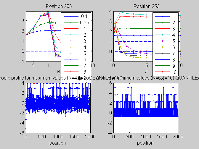
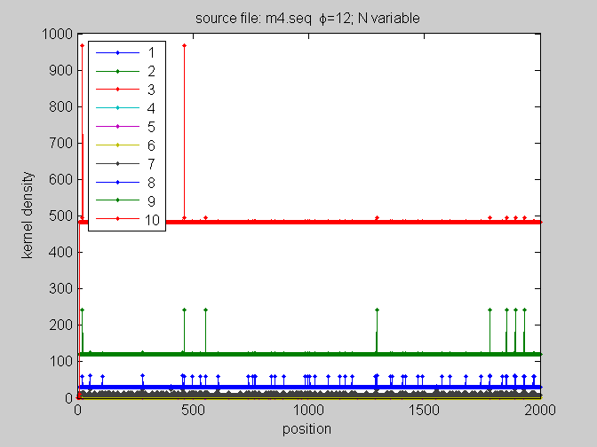
[KM,Ns,phis]=fill_kernel3D(cf); %use default parameters (forward counts)

%study a particular N=6 for all phis
figure;
plot(squeeze(KM(6,:,:))','.-');
xlabel('position');
ylabel('kernel density');
title([fasta.title '  N=6; \phi variable']);
legend(num2str((1:10)'),2);

% %study KM=f(pos,Ns) for fixed phis
% for i=1:12;
% figure
% plot(squeeze(KM(:,i,:))','.-');
% xlabel('position');
% ylabel('kernel density');
% title([fasta.title '  \phi=' num2str(i) '; N variable']);
% legend(num2str((1:10)'),2);
% end

%study KM=f(pos,Ns) for fixed phis

figure
plot(squeeze(KM(:,12,:))','.-');
xlabel('position');
ylabel('kernel density');
title([fasta.title '  \phi=' num2str(12) '; N variable']);
legend(num2str((1:10)'),2);

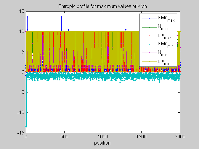
KMn=normKM(KM,1);
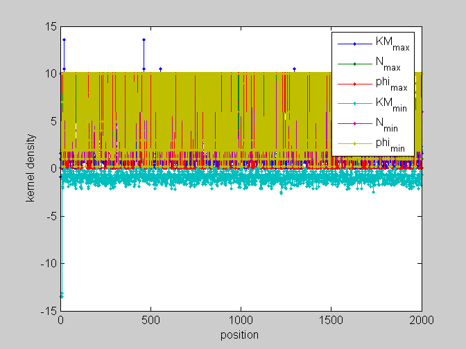
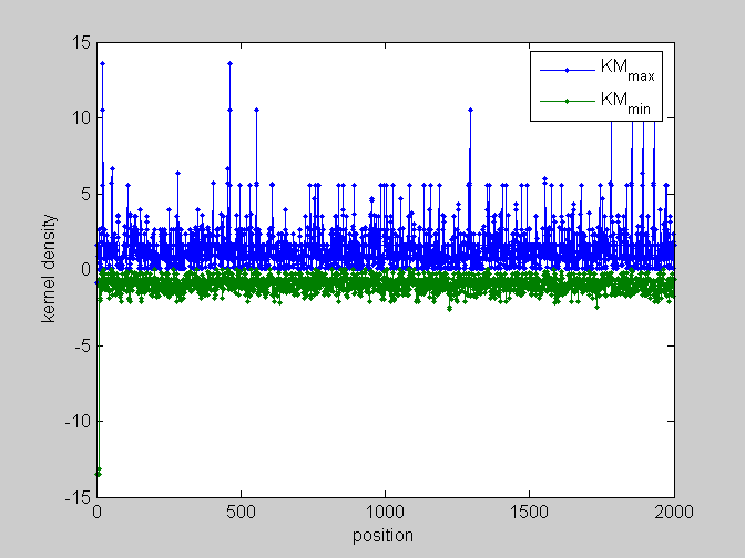
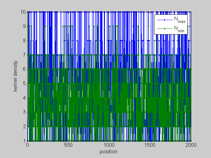
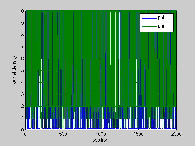
[pos,code]=find_scale(KMn,Ns,phis);
%...and plot
figure;plot(pos,'.-');legend(code);xlabel('position');ylabel('kernel density')
%partial plots
figure;plot(pos(:,[1,4]),'.-');legend(code([1,4]));xlabel('position');ylabel('kernel density')
figure;plot(pos(:,[2,5]),'.-');legend(code([2,5]));xlabel('position');ylabel('kernel density')
figure;plot(pos(:,[3,6]),'.-');legend(code([3,6]));xlabel('position');ylabel('kernel density')
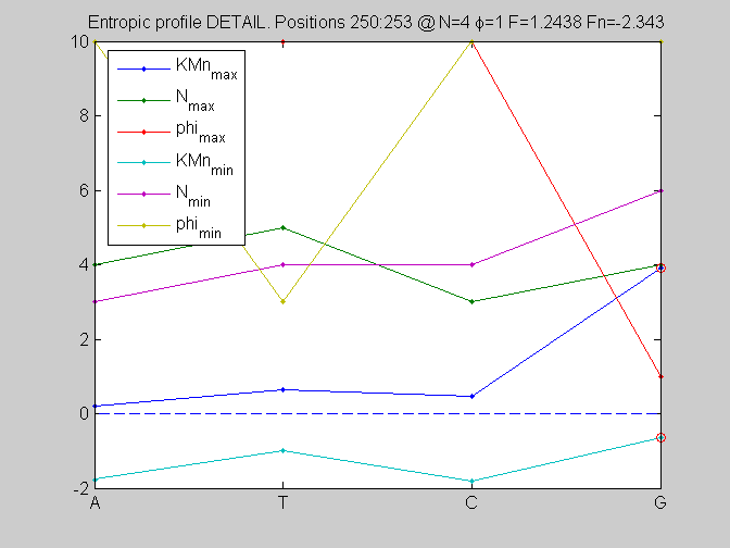
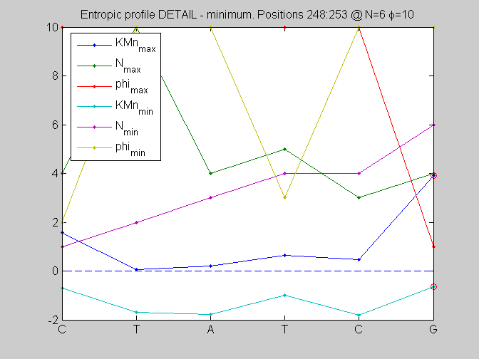
local_study(253,KMn,phis,Ns,pos,L,seq,KM);
F =

    1.2438


Fn =

   -2.3430