ROSETTA

Contents:
• Part I - Underlying urban grid
• Part II - Adding randomness and variability
• Part III - Modelling height change

In this tutorial we will be looking at how to use Rosetta to generate examples of cities structured with a grid plan. A grid plan is a type of urban structure where streets and building run alongside each other at right angles. It is a method of urban planning that dates back to the Classic period and is still much in use today.

The method we will be using to model one such example of city relies on recursion to create the underlying grid structure that we will afterwards populate with buildings. There are obviously other methods of achieving the final result and we encourage the reader to think and experiment with other methods.

In Figure 1 you can see an example of a city that displays the type of structure we are aiming to model.

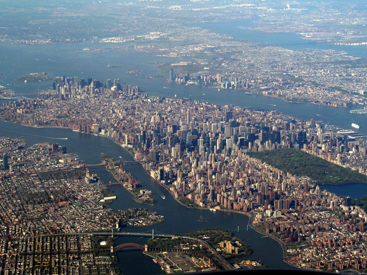
FIGURE 1 | Bird’s Eye view of the city of New York. Photography by Art Siegel

The city of New York is a good example of a city structure with an orthogonal plan. We can see that the city is organized in rectangular blocks, each containing a certain number of buildings.

Let’s take a moment to think on the best way to tackle the modelling of this type of city: we want to use recursion to generate a certain number of city blocks that, together, form the city grid. For that we need to create a function that creates one such block, inserted on a point p, and then create another function that recursively takes one block and generates an entire row of m blocks. Finally, we will define yet another function that takes one generated row and recursively duplicates it n number of times up to complete the grid. The last thing we will need is a function the models a building. For this, and for the time being, we will consider that a building has a square footprint, with length l, and that it occupies the entire area of a city block. Each block is spaced s units from the others thus defining the streets between them. Figure 2 shows a schematic drawing of this paradigm.

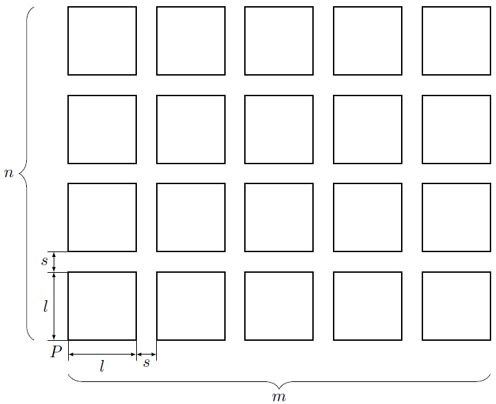
FIGURE 2 | Quick top view schematic of a grid city

So, let’s begin by launching DrRacket, loading Rosetta and choosing the CAD application you wish to use:

#lang racket

(require (planet aml/rosetta))
(backend rhino5)

Because we are considering that the buildings take up the entire block area we needn’t worry about modelling a block with sidewalks and so forth. We need only to create a building with the same dimensions as the block. Let’s define a function called building that models one building with parameters the insertion point p, the length l and height h. To use these parameters the most appropriate tool to use is the box function. The function building is thus defined:

(define (building p l h)
  (box p l l h))

Next we need to define a function that takes one building and recursively creates an entire row of buildings along the x direction. We will call this new function buildings-row and it will have as parameters the row insertion point p, the length, and height of the building (l and h respectively), the spacing between each building s and the number of building we wish to generate (m-buildings):

(define (buildings-row p l h s m-buildings)
  (if (= m-buildings 0)
      #t
      (begin
        (building p l h)
        (buildings-row (+x p (+ l s)) l h s (- m-buildings 1)))))

Let’s test this function out and see what it can create:

(buildings-row (xy 0 0) 100 400 40 8)

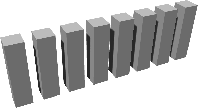
FIGURE 3 | A row of generated buildings

So far so good. We have a function that can model a very simply building and another function that can create a row of buildings. What we want to do now is take one row of buildings and create another recursion, this time along the y direction, to model an entire orthogonal grid of buildings. Let’s define this next function, called city-grid, with the same parameters as the previous function but adding the additional parameter - n-streets, that specifies how many rows of buildings we wish to create:

(define (city-grid p l h s n-streets m-buildings)
  (if (= n-streets 0)
      #t
      (begin
        (buildings-row p l h s m-buildings)
        (city-grid (+y p (+ l s)) l h s (- n-streets 1) m-buildings))))

In Figure 4 we can see the result of our work so far:

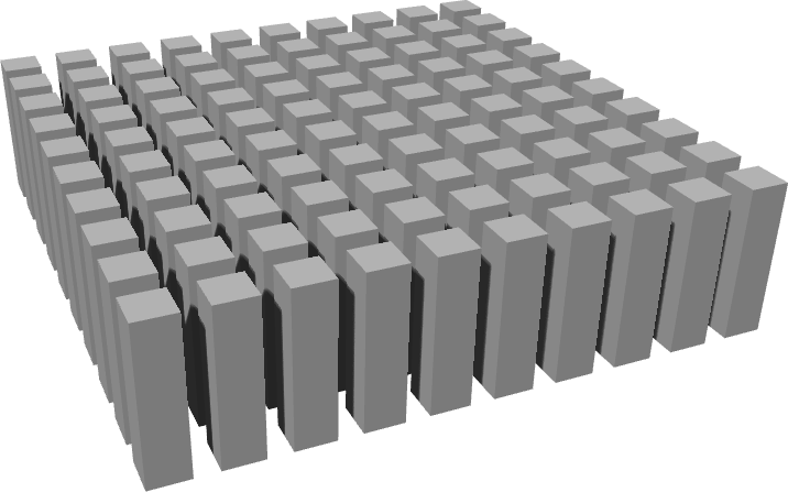
FIGURE 4 | A grid of generated buildings

At this point we can generate a rectangular grid of buildings but this hardly resembles a realistic city. What gives the impression of randomness in a cityscape is, between other factors, the variation of heights observable in all buildings.

Using Rosetta we can easily introduce this element of randomness in our functions. In fact, the only function that needs to be modified is the building function. The parameter h is at the moment a set input we specify and all buildings generated by the function building will create the same result each time the function is computed. Introducing the function random-range we can either make the height vary between a specific range or we can have a random-range function generate a scale factor that will be applied to the h parameter:

(define (building p l h)
  (box p l l (* (random-range 0.1 1.0) h)))

Now if we run the function city-grid again we can see how much the final result has changed simply by adding a bit of randomness:

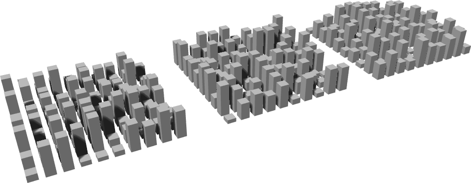
FIGURE 5 | Grid of buildings with random heights

The final result looks much nicer and closer to reality but it still lacks a certain degree of variability. There is another aspect we can change in our functions and that is to have more than one possible shape of building. Let’s consider that we have two types of buildings in our city: a box-shaped building (building0) and a cylinder-shaped building (building1). The previous function building will be renamed building0 and we will define a new function for the building1 that uses Rosetta’s function cylinder to model it. This function receives as parameters the base centre point and radius but because it is not convenient to introduce more parameters than those we already have we shall define the cylinder’s radius in terms of the parameter l:

(define (building1 p l h)
  (cylinder (+xy p (/ l 2.0) (/ l 2.0))
            (/ l 2.0) (* (random-range 0.1 1.0) h)))

Now, in order to have the cylindrical building pop up randomly each time we run the program city-grid, we need to make sure, somewhere, there is a conditional statement that makes the choice of which building to place down. One possibility is to have a generator of random numbers between, for example, 0 and 5 to have a ratio of 20 to 80% of each building, and create a conditional statement that states “If the number generated is 0 then place down a building1. Otherwise, place down a building0.” Let’s try to implement this in the building function:

(define (building p l h)
  (if (= (random 5) 0)
      (building1 p l h)
      (building0 p l h)))

If we test the function city-grid again we can see that it randomly chooses between a box-shaped building and a cylindrical building.

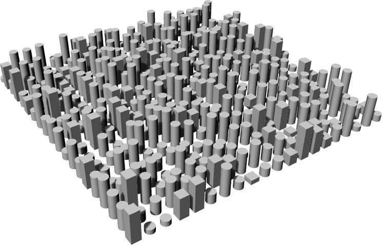
FIGURE 6 | City with of different buildings

With this change the city-grid will now generate an even more random and realistic city than before, this time with variable heights and different types of buildings.

We could apply some more randomness to our buildings though, since most high-rise buildings have a more intricate shape than mere boxes or cylinders. In Figure 7 we can see this clearly in the city of Manhattan.

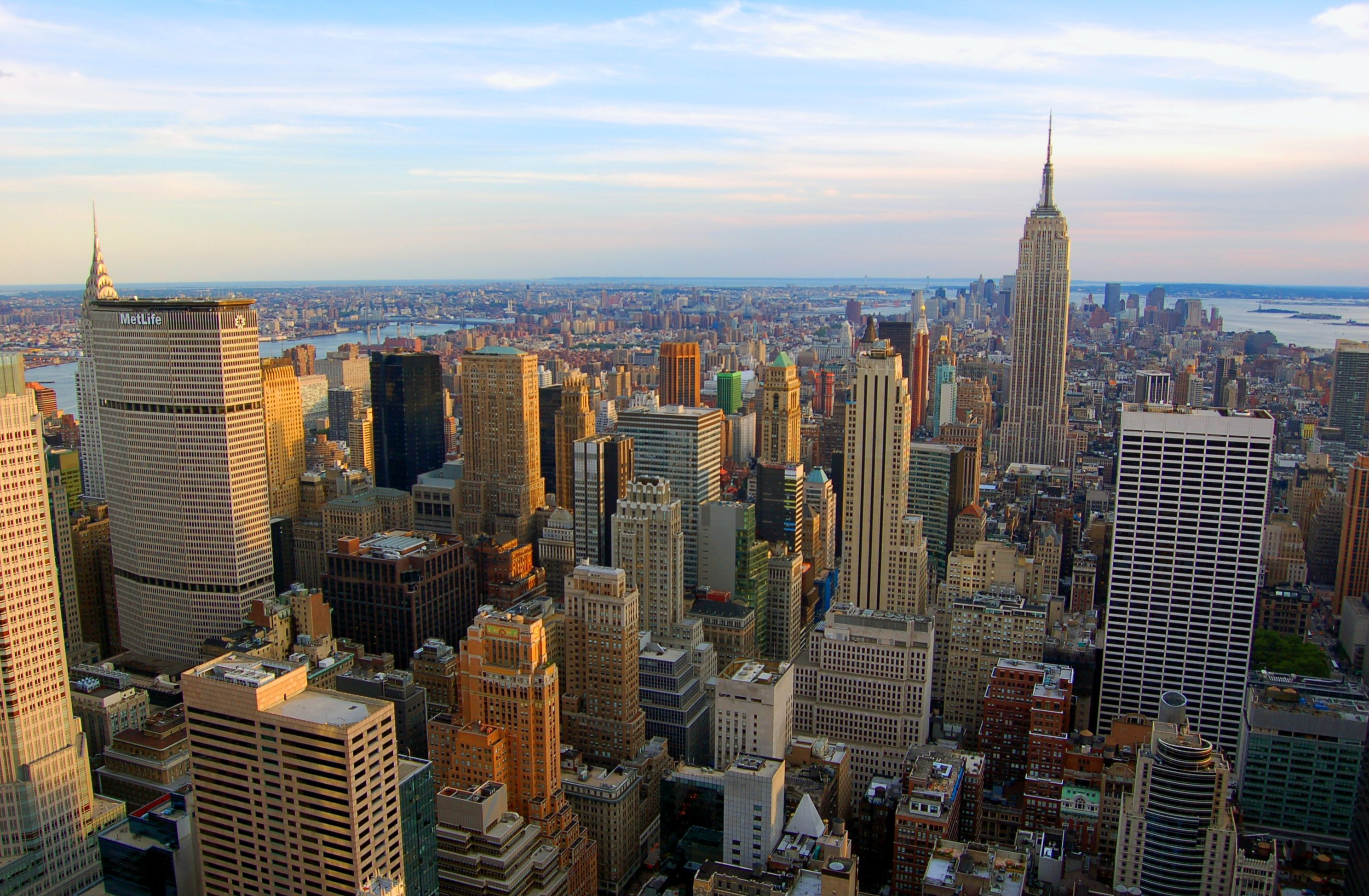
FIGURE 7 | The city of Manhattan. Photography by James K. Poole

One thing we could do, for example, is to make each building be composed of several smaller segments as it rises. Let’s suppose that if a building has a length l and a height h then it can be composed of 0 to 6 stacked blocks, each with a height that’s between 20 to 80% of h and a length and width between 70 and 100% of l. We will take the box-shaped building and try to implement this, first creating the function building0-blocks for creating stacked blocks and a new building0 function where the n-blocks parameter will be randomly chosen:

(define (building0-blocks p l w h n-blocks)
  (let* ((top-h (* (random-range 0.2 0.8) h))
         (top-l (* (random-range 0.7 1.0) l))
         (top-w (* (random-range 0.7 1.0) w))
         (top-p (+xyz p (/ (- l top-l) 2.0) (/ (- w top-w) 2.0) top-h)))
    (if (= n-blocks 1)
        (box p l w h)
        (begin
          (box p l w top-h)
          (building0-blocks top-p top-l top-w top-h (- n-blocks 1))))))

(define (building0 p l h)
  (building0-blocks p l l h (random-range 1 6)))

Note that to make our job easier we defined some local variables: top-h, the height of the first block that’s between 20 and 80% of h; top-l and top-w which represent the length and width of each stacked block; and top-p which is the new insertion point for the recursion. The stopping condition for the recursion is when the number of stacked blocks is 1, in which case only one box is created. Let’s now create the same definition but for the cylindrical building:

(define (building1-blocks p l h n-blocks)
  (let* ((top-h (* (random-range 0.2 0.8) h))
         (top-l (* (random-range 0.7 1.0) l))
         (top-p (+xyz p (/ (- l top-l) 2.0) (/ (- l top-l) 2.0) top-h)))
    (if (= n-blocks 1)
        (cylinder (+xy p (/ l 2.0) (/ l 2.0)) (/ l 2.0) h)
        (begin
          (cylinder (+xy p (/ l 2.0) (/ l 2.0)) (/ l 2.0) top-h)
          (building1-blocks top-p top-l top-h (- n-blocks 1))))))

(define (building1 p l h)
  (building1-blocks p l h (random-range 1 6)))

Finally we are only left with changing the building-row and city-grid functions to accommodate these changes:

(define (buildings-row p l h s m-buildings )
  (if (= m-buildings 0)
      #t
      (begin
        (building p l h)
        (buildings-row (+x p (+ l s)) l h s (- m-buildings 1)))))

(define (city-grid p l h s n-streets m-buildings)
  (if (= n-streets 0)
      #t
      (begin
        (buildings-row p l h s m-buildings)
        (city-grid (+y p (+ l s)) l h s (- n-streets 1) m-buildings))))

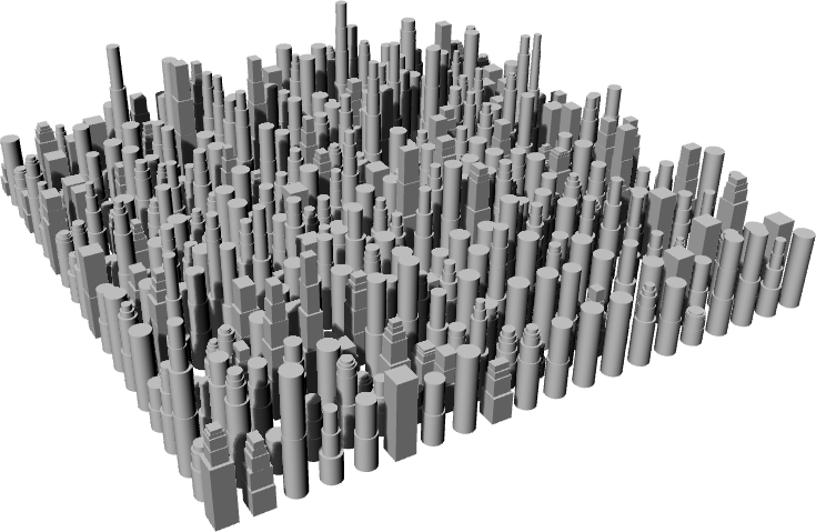
FIGURE 8 | Randomly generated city

One final characteristic of cities which we will attempt to simulate is how cities tend to have clusters of relatively high buildings, often corresponding to the central business district, and, as the cities extend outwards towards the suburbs, the height tends to decrease. To model this behaviour we can use a bi-dimensional Gaussian distribution to affect the height parameter.

A bi-dimensional Gaussian distribution is defined as:

Where f is the height factor, x0 and y0 are the coordinates of the highest point in the Gaussian surface and sigma0 and sigma1 are the factors that affect the bi-dimensional stretch of that surface. To make things easier, let’s consider that the business district is located at the coordinates (0;0) and that sigmax = sigmay = 45l, where l is a block’s length.

Let’s first define a function that translates the bi-dimensional Gaussian distribution according to the formula above:

(define (gaussian-2d x y sigma)
  (exp (- (+ (expt (/ x sigma) 2)
             (expt (/ y sigma) 2)))))

And then introduce that function in the building function and have it affect the height parameter:

(define (building p l h)
  (set! h (* h (max 0.1 (gaussian-2d  (cx p) (cy p) (* 45.0 l)))))
  (if (= (random 5) 0)
      (building1 p l h)
      (building0 p l h)))

Let’s have a look at what the function city-grid can now do. For added effect we changed the display mode of the viewport from “Shaded” to “Rendered” and increased the number of generated buildings to 40 in each direction:

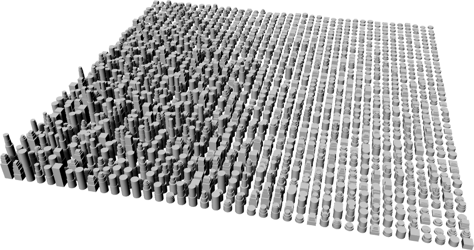
FIGURE 9 | A random city with suburbs and one business district

Lastly, and something that is also common in many cities, we may want our cities to have more than one central business district. If before we used a Gaussian distribution to control the height of buildings in one direction then we can use the same strategy and combine more than one distribution to create several clusters of business districts, i.e., at each point the height of a building will be the maximum height of each Gaussian distribution:

(define (building p l h)
  (let ((coef (max
               (gaussian-2d (- 500 (cx p)) (- 500 (cy p)) (* 11 l))
               (gaussian-2d (- 2000 (cx p)) (- 5500 (cy p)) (* 14 l))
               (gaussian-2d (- 4500 (cx p)) (- 2500 (cy p)) (* 13 l)))))
  (when (> coef 0.005)
    (set! h (* h (max coef 0.005)))
    (if (= (random 5) 0)
        (building1 p l h)
        (building0 p l h)))))

Note that in each Gaussian distribution we specify the location of each business district in terms of how distant they are from p. The minimum coefficient value that we are considering can also be changed to produce different results:

(city-grid (xy 0 0) 100 400 40 40 40)

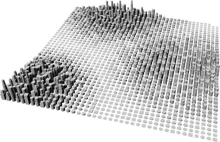
FIGURE 10 | A random city with suburbs and three business districts

In this tutorial we looked at how to generate a seemingly random urban grid of buildings using recursion, the random-range function to introduce randomness and finally how to use a distribution function to control a parameter. The final result could be enhanced by adding even more detail to the buildings and city blocks (add windows, create more intricately shaped buildings, model sidewalks, create empty areas for parks and plazas, use other types of distribution functions, etc.). In part II we will look at another method of generating random cities, this time not using recursion but surface processing and mapping techniques instead. This will allow the generation of very interesting cities with a great degree of complexity.