ROSETTA

Contents:
• Part I - Recursion
• Part II - Shape Algebras

In this brief guide we will introduce you to the basic fundamentals or recursion. Recursion is one of the most powerful mechanisms in computer science but not limited to it. In fact, if you look around you, you’ll be surprised by the shear amount of recursion that exists in the real world: trees, plants, stairs, a coastline, reflections in a mirror, trusses, cities, the structure of the human DNA, the process of natural evolution, all are examples or recursion. More mathematically speaking though, we can define a recursive function as a function that is defined in terms of itself or, in other words, a function that calls itself during its evaluation. So the main idea is that the solution to a particular problem depends on progressively solving smaller and less complex sub-problems.

Here’s an example: we wish to design a staircase to cover a certain height. A staircase is nothing more than a set of steps, placed so as to create the overall body of a staircase. So we could say that in order to design a staircase we could decompose that problem into a smaller problem which is to design one step first and then create all the remaining steps minus one. An even simpler and smaller problem would be to not design the staircase at all. This leads us to the following paradigm: if we don’t have to create any steps then we don’t need to create anything and the problem is solved. Otherwise, we must create at least one step. Finally, and if we are feeling lazy, we tell someone else to create the rest of the steps while we have a rest.

All recursive programs have the following structure:

• A basic case, also called the stopping condition, to which we have an immediate solution to;
• A less basic case, also called recursive case, which transforms the original problem into slightly simpler sub-problem.

If we follow this structure a recursive program will usually have the following pattern:

• We start by testing basic cases;
• We recursively invoke the program with a sub-problem that is closer to the basic case;
• We use the result of the last recursion to calculate the result of the next invocation.

The most reoccurring mistakes associated with recursive functions are:

• Not detecting the most basic case (stopping condition);
• The complexity of the problem is not reduced throughout the recursion;
• Not using the result of the recursion to obtain the desire effect.

Taking the example of the staircase again, let’s create a function capable of modelling it. We have some planning to do first: we want to create a staircase starting at a point p, with steps having a length of l and a height of h and with a total number of n steps.

A said earlier, we can decompose this problem of creating a staircase with n steps into the simpler sub-problem of creating a staircase with n-1 steps. Even simpler, a staircase with (n – 2), and a staircase with (n – 3), so on and so forth, until the point in which we have (n – n) which is zero. This last case is in fact the stopping condition for our recursive function – when the parameter n equals 0 then we need to stop creating steps and our staircase is complete. To implement this condition we can use Racket’s function if which has the following syntax:

(if logical expression
    consequential expression
    alternative expression)

Which translates to: if the logical expression is true than evaluate the consequential expression. Otherwise, evaluate the alternative expression. In our case, the logical expression will be (= n 0), or alternatively (zero? n), the consequential expression will be to do nothing and in Racket we can use the Boolean value #t to mean that, and our alternative expression will be to create one step and then create all the others minus 1.

Now, paying attention to what we’ve just said and to the syntax of the if statement we see a small problem. Our alternative expression is actually two things (create one step and create the remaining steps minus 1) but the syntax only supports one alternative expression. To work around this problem Racket provides the function begin which allows the combination of a number of expressions into a single one, sequentially evaluating them. The syntax will thus be:

(if logical expression
    consequential expression
    (begin
      first alternative expression
      second alternative expression))

So, a first sketch of our recursive staircase function would look something like this:

(define (staircase p l h n)
  (if (= n 0)
      #t
      (begin
        ...
        ...)))

We know that the consequential expression is to draw one step first. For that we can use the line function and input the necessary coordinates for drawing the staircase’s rise and thread:

(define (staircase p l h n)
  (if (= n 0)
      #t
      (begin
        (line p (+xy p 0 h) (+xy p l h))
        ...)))

Finally, the function needs to call upon itself for creating the remaining steps but we know that are two things that need to change: the point p must now be (+xy p l h) and that n must now be (- n 1):

(define (staircase p l h n)
  (if (= n 0)
      #t
      (begin
        (line p (+xy p 0 h) (+xy p l h))
        (staircase (+xy p l h) l h (- n 1)))))

We can see the result in Figure 1:

FIGURE 1 | A staircase.with10 steps

Here we see one of the big advantages of using recursion. The alternative to modelling this staircase without recursion would be to manually design all the steps but would you really want to go through all that trouble? And even if in CAD applications you can use certain operations, such as arrays, to create multiple copies of an element almost effortlessly consider this particular case: we want the rise and thread of each step to decrease along the staircase. To do this manually would be a lot of work but using our recursive function we only need to multiply the length l and height h by a factor:

(define (staircase p l h n)
  (if (= n 0)
      #t
      (begin
        (line p (+xy p 0 h) (+xy p l h))
        (staircase (+xy p l h) (* l 0.8) (* h 0.8) (- n 1)))))

The result is visible in Figure 2:

FIGURE 2 | A progressively smaller staircase.with10 steps

Or another different example: we want to draw circles along the positive vertical and horizontal direction that are in a geometric progression of ratio f. Here we could use a different stopping condition; we don’t want to specify how many circles we wish to draw so, alternatively, we could say we want to stop creating circles at the point where the last created circle has a radius below a certain value. This new function, which for lack of a better name we will call circles, will look something like this:

(define (circles p r f)
  (if (< r 0.2)
      #t
      (begin
        (circle p r)
        (circles (+pol p r 0) (* r f) f)
        (circles (+pol p r pi/2) (* r f) f))))

Where p is the insertion point of the first circle, r is the radius of the first circle and f is the factor to which we multiply by the radius during the recursion. That radius will therefore decrease during the recursion at the point where it will be below the value 0.2, point at which the function will stop. The result is in Figure 3:

FIGURE 3 | A series of circles in a geometric progression of 1/2

We’d like to leave you with another example and this time we will use 3D geometry. If you look at the example of circles you’ll see that, during the recursion, the function reproduces those three lines of code after the begin for each step. That is why the function generates circles in both horizontal and vertical directions thus creating that diagonal appearance. If we wanted to only create a line of circles in both directions then we’d have to split the function in two. We would need to have a recursive function for creating a line of circles in the horizontal direction and another recursive function that creating the vertical line of circles. This way of working is common when working with recursive functions. In many cases, to achieve what we want, we can’t have just one miracle function that solves everything. Another example would be a standard rectangular grid where we have a series of rows and columns.

Let’s consider we want to place cuboids in a grid fashion with a height changing decreasing along the recursion. To model this we will have to first model one row of cuboids. If p is the row insertion point, l, w and h are respectively the cuboids’ length, width and height, s is the spacing between cuboids and e-x is the number of cuboids to place down then our cuboids-row will look something like this:

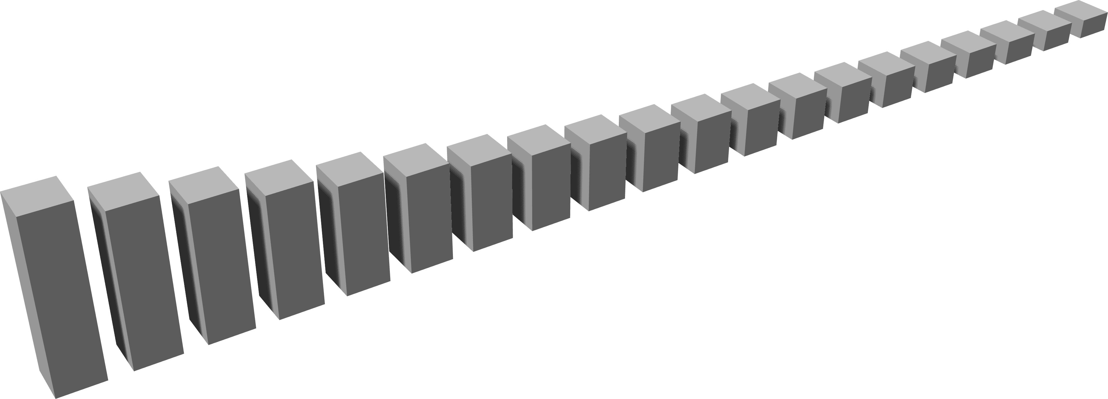
(define (cuboids-row p e-x l w h s)
  (if (= e-x 0)
      #t
      (begin
        (right-cuboid p l w h)
        (cuboids-row (+x p (+ l s)) (- e-x 1) l w (* h 0.9) s))))

The stopping condition is when the e-x parameter reaches the value 0. During the recursion the function creates e-x cuboids minus one and the height is multiplied by 0.9 to have the cuboids’ height decrease along the recursion process.

FIGURE 4 | A row of cuboids

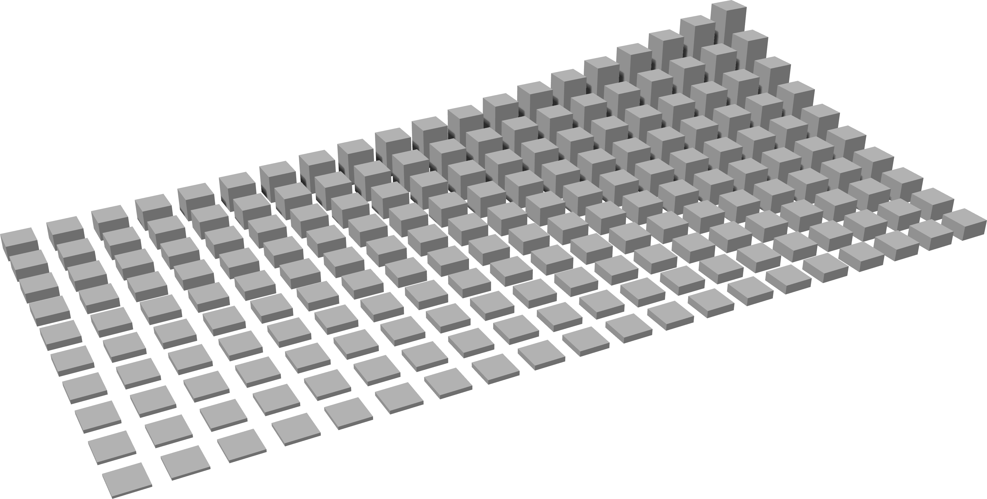
We now want to create the rest of the grid which translate into recursively creating rows of cuboids in the vertical (y axis) direction. Once more the stopping condition is when the number of rows – e-y – reaches 0. The height is also multiplied by a reduction factor:

(define (cuboids-grid p e-x e-y l w h s)
  (if (= e-y 0)
      #t
      (begin
        (cuboids-row p e-x l w h s)
        (cuboids-grid (+y p (+ w s)) e-x (- e-y 1) l w (* h 0.8) s))))

FIGURE 5 | A grid of cuboids

This is intended to be just a quick guide to get you started with recursion since Rosetta doesn’t offer particular functions to work with this. Due to its importance in computer science most programming languages, to which Racket is no exception, already have the necessary means to handle recursion so this guide was just to show you how to adapt this kind of behaviour in a meaningful way by producing geometry we can see and use later. In the misc section of these intermediate tutorials you will find more examples of recursion.

In the next tutorial we will discuss randomness and state which, coupled with recursion, can produce very interesting results. Click the link below when you’re ready.